Introduction to scRNA-seq integration
Compiled: May 22, 2026
Source:vignettes/integration_introduction.Rmd
integration_introduction.RmdIntroduction to scRNA-seq integration
Integration of single-cell sequencing datasets, for example across experimental batches, donors, or conditions, is often an important step in scRNA-seq workflows. Integrative analysis can help to match shared cell types and states across datasets, which can boost statistical power, and most importantly, facilitate accurate comparative analysis across datasets. In previous versions of Seurat we introduced methods for integrative analysis, including our ‘anchor-based’ integration workflow. Many labs have also published powerful and pioneering methods, including Harmony and scVI, for integrative analysis. Please see our Integrating scRNA-seq data with multiple tools vignette.
Integration goals
The following tutorial is designed to give you an overview of the kinds of comparative analyses on complex cell types that are possible using the Seurat integration procedure. Here, we address a few key goals:
- Identify cell subpopulations that are present in both datasets
- Obtain cell type markers that are conserved in both control and stimulated cells
- Compare the datasets to find cell-type specific responses to stimulation
Setup the Seurat objects
For convenience, we distribute this dataset through our SeuratData package.
# install dataset
InstallData("ifnb")
The object contains data from human PBMC from two conditions,
interferon-stimulated and control cells (stored in the stim
column in the object metadata). We will aim to integrate the two
conditions together, so that we can jointly identify cell subpopulations
across datasets, and then explore how each group differs across
conditions
In previous versions of Seurat, we would require the data to be represented as two different Seurat objects. In Seurat v5, we keep all the data in one object, but simply split it into multiple ‘layers’. To learn more about layers, check out our Seurat object interaction vignette.
Perform analysis without integration
We can first analyze the dataset without integration. The resulting clusters are defined both by cell type and stimulation condition, which creates challenges for downstream analysis.
# run standard analysis workflow
ifnb <- NormalizeData(ifnb)
ifnb <- FindVariableFeatures(ifnb)
ifnb <- ScaleData(ifnb)
ifnb <- RunPCA(ifnb)
ifnb <- FindNeighbors(ifnb, dims = 1:30, reduction = "pca")
ifnb <- FindClusters(ifnb, resolution = 2)
## Modularity Optimizer version 1.3.0 by Ludo Waltman and Nees Jan van Eck
##
## Number of nodes: 13999
## Number of edges: 555146
##
## Running Louvain algorithm...
## Maximum modularity in 10 random starts: 0.8153
## Number of communities: 26
## Elapsed time: 2 seconds
ifnb <- RunUMAP(ifnb, dims = 1:30, reduction = "pca", reduction.name = "umap.unintegrated")
DimPlot(ifnb, reduction = "umap.unintegrated", group.by = c("stim", "seurat_clusters"))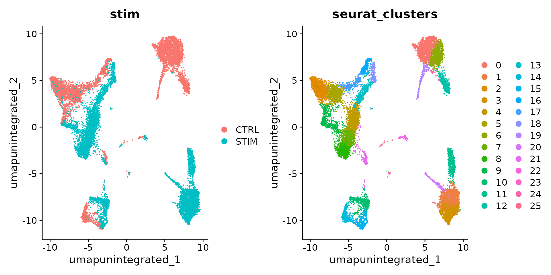
Perform integration
We now aim to integrate data from the two conditions, so that cells from the same cell type/subpopulation will cluster together.
We often refer to this procedure as intergration/alignment. When aligning two genome sequences together, identification of shared/homologous regions can help to interpret differences between the sequences as well. Similarly for scRNA-seq integration, our goal is not to remove biological differences across conditions, but to learn shared cell types/states in an initial step - specifically because that will enable us to compare control stimulated and control profiles for these individual cell types.
The Seurat v5 integration procedure aims to return a single
dimensional reduction that captures the shared sources of variance
across multiple layers, so that cells in a similar biological state will
cluster. The method returns a dimensional reduction
(i.e. integrated.cca) which can be used for visualization
and unsupervised clustering analysis. For evaluating performance, we can
use cell type labels that are pre-loaded in the
seurat_annotations metadata column.
ifnb <- IntegrateLayers(object = ifnb, method = CCAIntegration, orig.reduction = "pca", new.reduction = "integrated.cca",
    verbose = FALSE)

# re-join layers after integration
ifnb[["RNA"]] <- JoinLayers(ifnb[["RNA"]])

ifnb <- FindNeighbors(ifnb, reduction = "integrated.cca", dims = 1:30)
ifnb <- FindClusters(ifnb, resolution = 1)
## Modularity Optimizer version 1.3.0 by Ludo Waltman and Nees Jan van Eck
##
## Number of nodes: 13999
## Number of edges: 590511
##
## Running Louvain algorithm...
## Maximum modularity in 10 random starts: 0.8452
## Number of communities: 18
## Elapsed time: 3 seconds
ifnb <- RunUMAP(ifnb, dims = 1:30, reduction = "integrated.cca")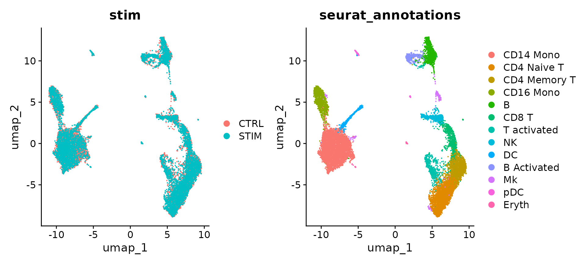
To visualize the two conditions side-by-side, we can use the
split.by argument to show each condition colored by
cluster.
DimPlot(ifnb, reduction = "umap", split.by = "stim")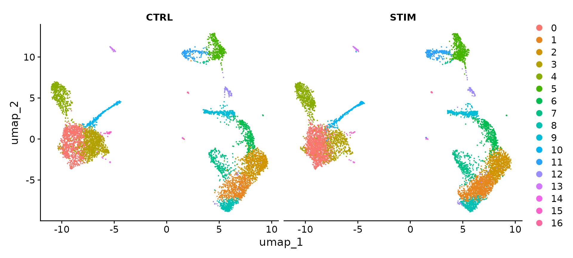
Identify conserved cell type markers
To identify canonical cell type marker genes that are conserved
across conditions, we provide the FindConservedMarkers()
function. This function performs differential gene expression testing
for each dataset/group and combines the p-values using meta-analysis
methods from the MetaDE R package. For example, we can calculated the
genes that are conserved markers irrespective of stimulation condition
in cluster 6 (NK cells).
Idents(ifnb) <- "seurat_annotations"
nk.markers <- FindConservedMarkers(ifnb, ident.1 = "NK", grouping.var = "stim", verbose = FALSE)
head(nk.markers)
## CTRL_p_val CTRL_avg_log2FC CTRL_pct.1 CTRL_pct.2 CTRL_p_val_adj
## GNLY 0 6.854586 0.943 0.046 0
## NKG7 0 5.358881 0.953 0.085 0
## GZMB 0 5.078135 0.839 0.044 0
## CLIC3 0 5.765314 0.601 0.024 0
## CTSW 0 5.307246 0.537 0.030 0
## KLRD1 0 5.261553 0.507 0.019 0
## STIM_p_val STIM_avg_log2FC STIM_pct.1 STIM_pct.2 STIM_p_val_adj max_pval
## GNLY 0 6.435910 0.956 0.059 0 0
## NKG7 0 4.971397 0.950 0.081 0 0
## GZMB 0 5.151924 0.897 0.060 0 0
## CLIC3 0 5.505208 0.623 0.031 0 0
## CTSW 0 5.240729 0.592 0.035 0 0
## KLRD1 0 4.852457 0.555 0.027 0 0
## minimump_p_val
## GNLY 0
## NKG7 0
## GZMB 0
## CLIC3 0
## CTSW 0
## KLRD1 0You can perform these same analysis on the unsupervised clustering
results (stored in seurat_clusters), and use these
conserved markers to annotate cell types in your dataset.
The DotPlot() function with the split.by
parameter can be useful for viewing conserved cell type markers across
conditions, showing both the expression level and the percentage of
cells in a cluster expressing any given gene. Here we plot 2-3 strong
marker genes for each of our 14 clusters.
Idents(ifnb) <- factor(Idents(ifnb), levels = c("pDC", "Eryth", "Mk", "DC", "CD14 Mono", "CD16 Mono",
    "B Activated", "B", "CD8 T", "NK", "T activated", "CD4 Naive T", "CD4 Memory T"))

markers.to.plot <- c("CD3D", "CREM", "HSPH1", "SELL", "GIMAP5", "CACYBP", "GNLY", "NKG7", "CCL5",
    "CD8A", "MS4A1", "CD79A", "MIR155HG", "NME1", "FCGR3A", "VMO1", "CCL2", "S100A9", "HLA-DQA1",
    "GPR183", "PPBP", "GNG11", "HBA2", "HBB", "TSPAN13", "IL3RA", "IGJ", "PRSS57")
DotPlot(ifnb, features = markers.to.plot, cols = c("blue", "red"), dot.scale = 8, split.by = "stim") +
    RotatedAxis()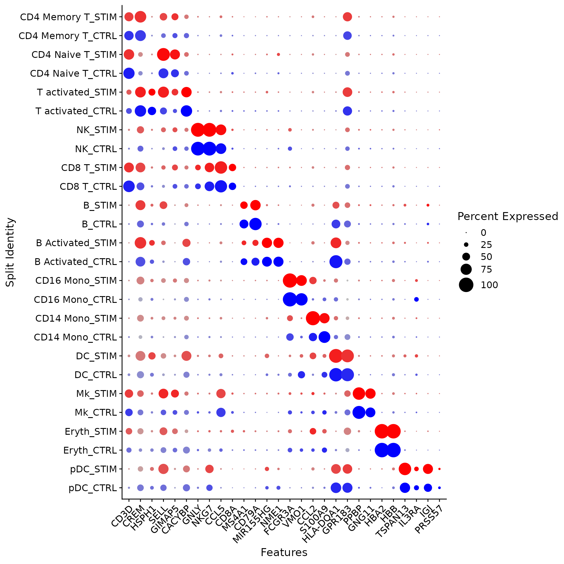
Identify differential expressed genes across conditions
Now that we’ve aligned the stimulated and control cells, we can start to do comparative analyses and look at the differences induced by stimulation.
We can aggregate cells of a similar type and condition together to
create “pseudobulk” profiles using the AggregateExpression
command. As an initial exploratory analysis, we can compare pseudobulk
profiles of two cell types (naive CD4 T cells, and CD14 monocytes), and
compare their gene expression profiles before and after stimulation. We
highlight genes that exhibit dramatic responses to interferon
stimulation. As you can see, many of the same genes are upregulated in
both of these cell types and likely represent a conserved interferon
response pathway, though CD14 monocytes exhibit a stronger
transcriptional response.
library(ggplot2)
library(cowplot)
theme_set(theme_cowplot())

aggregate_ifnb <- AggregateExpression(ifnb, group.by = c("seurat_annotations", "stim"), return.seurat = TRUE)
genes.to.label = c("ISG15", "LY6E", "IFI6", "ISG20", "MX1", "IFIT2", "IFIT1", "CXCL10", "CCL8")

p1 <- CellScatter(aggregate_ifnb, "CD14 Mono_CTRL", "CD14 Mono_STIM", highlight = genes.to.label)
p2 <- LabelPoints(plot = p1, points = genes.to.label, repel = TRUE)

p3 <- CellScatter(aggregate_ifnb, "CD4 Naive T_CTRL", "CD4 Naive T_STIM", highlight = genes.to.label)
p4 <- LabelPoints(plot = p3, points = genes.to.label, repel = TRUE)

p2 + p4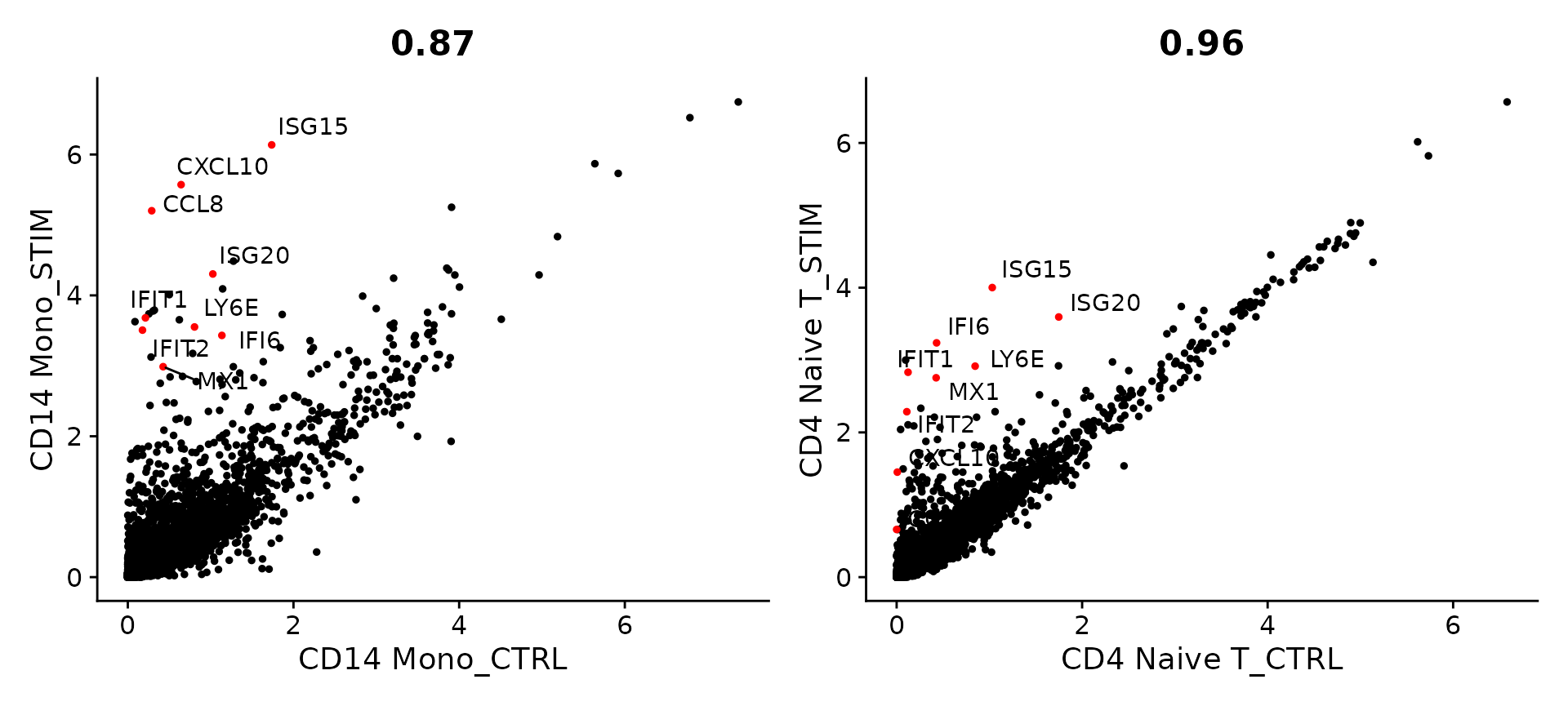
We can now ask what genes change in different conditions for cells of
the same type. First, we create a column in the meta.data slot to hold
both the cell type and stimulation information and switch the current
ident to that column. Then we use FindMarkers() to find the
genes that are different between stimulated and control B cells. Notice
that many of the top genes that show up here are the same as the ones we
plotted earlier as core interferon response genes. Additionally, genes
like CXCL10 which we saw were specific to monocyte and B cell interferon
response show up as highly significant in this list as well.
Please note that p-values obtained from this analysis should be interpreted with caution, as these tests treat each cell as an independent replicate, and ignore inherent correlations between cells originating from the same sample. As discussed here, DE tests across multiple conditions should expressly utilize multiple samples/replicates, and can be performed after aggregating (‘pseudobulking’) cells from the same sample and subpopulation together. We do not perform this analysis here, as there is a single replicate in the data, but please see our vignette comparing healthy and diabetic samples as an example for how to perform DE analysis across conditions.
ifnb$celltype.stim <- paste(ifnb$seurat_annotations, ifnb$stim, sep = "_")
Idents(ifnb) <- "celltype.stim"
b.interferon.response <- FindMarkers(ifnb, ident.1 = "B_STIM", ident.2 = "B_CTRL", verbose = FALSE)
head(b.interferon.response, n = 15)
## p_val avg_log2FC pct.1 pct.2 p_val_adj
## ISG15 5.387767e-159 5.0588481 0.998 0.233 7.571429e-155
## IFIT3 1.945114e-154 6.1124940 0.965 0.052 2.733468e-150
## IFI6 2.503565e-152 5.4933132 0.965 0.076 3.518260e-148
## ISG20 6.492570e-150 3.0549593 1.000 0.668 9.124009e-146
## IFIT1 1.951022e-139 6.2320388 0.907 0.029 2.741772e-135
## MX1 6.897626e-123 3.9798482 0.905 0.115 9.693234e-119
## LY6E 2.825649e-120 3.7907800 0.898 0.150 3.970885e-116
## TNFSF10 4.007285e-112 6.5802175 0.786 0.020 5.631437e-108
## IFIT2 2.672552e-108 5.5525558 0.786 0.037 3.755738e-104
## B2M 5.283684e-98 0.6104044 1.000 1.000 7.425161e-94
## PLSCR1 4.634658e-96 3.8010721 0.793 0.113 6.513085e-92
## IRF7 2.411149e-94 3.1992949 0.835 0.187 3.388388e-90
## CXCL10 3.708508e-86 8.0906108 0.651 0.010 5.211566e-82
## UBE2L6 5.547472e-83 2.5167981 0.851 0.297 7.795863e-79
## PSMB9 1.716262e-77 1.7715351 0.937 0.568 2.411863e-73Another useful way to visualize these changes in gene expression is
with the split.by option to the FeaturePlot()
or VlnPlot() function. This will display FeaturePlots of
the list of given genes, split by a grouping variable (stimulation
condition here). Genes such as CD3D and GNLY are canonical cell type
markers (for T cells and NK/CD8 T cells) that are virtually unaffected
by interferon stimulation and display similar gene expression patterns
in the control and stimulated group. IFI6 and ISG15, on the other hand,
are core interferon response genes and are upregulated accordingly in
all cell types. Finally, CD14 and CXCL10 are genes that show a cell type
specific interferon response. CD14 expression decreases after
stimulation in CD14 monocytes, which could lead to misclassification in
a supervised analysis framework, underscoring the value of integrated
analysis. CXCL10 shows a distinct upregulation in monocytes and B cells
after interferon stimulation but not in other cell types.
FeaturePlot(ifnb, features = c("CD3D", "GNLY", "IFI6"), split.by = "stim", max.cutoff = 3, cols = c("grey",
    "red"), reduction = "umap")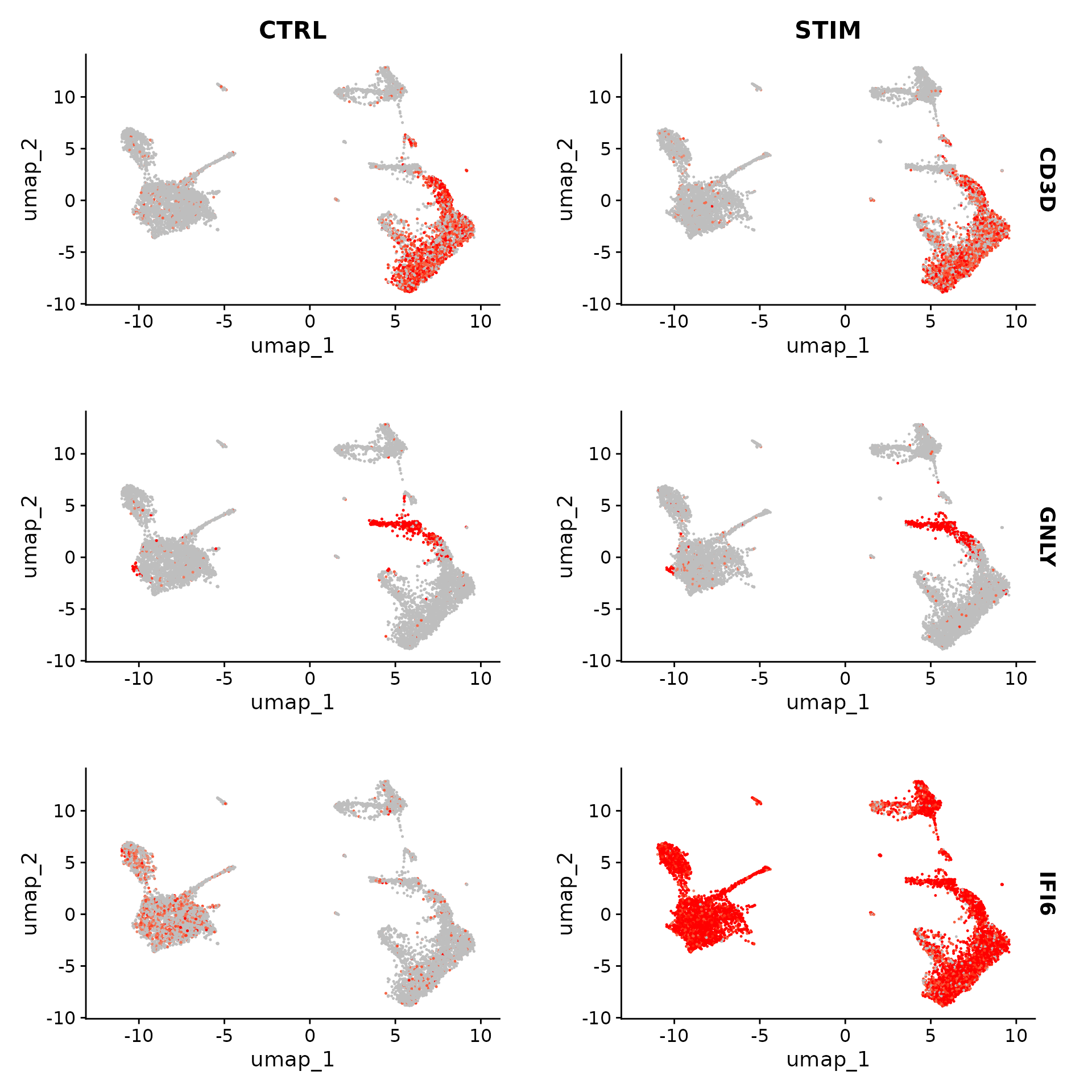
plots <- VlnPlot(ifnb, features = c("LYZ", "ISG15", "CXCL10"), split.by = "stim", group.by = "seurat_annotations",
    pt.size = 0, combine = FALSE)
wrap_plots(plots = plots, ncol = 1)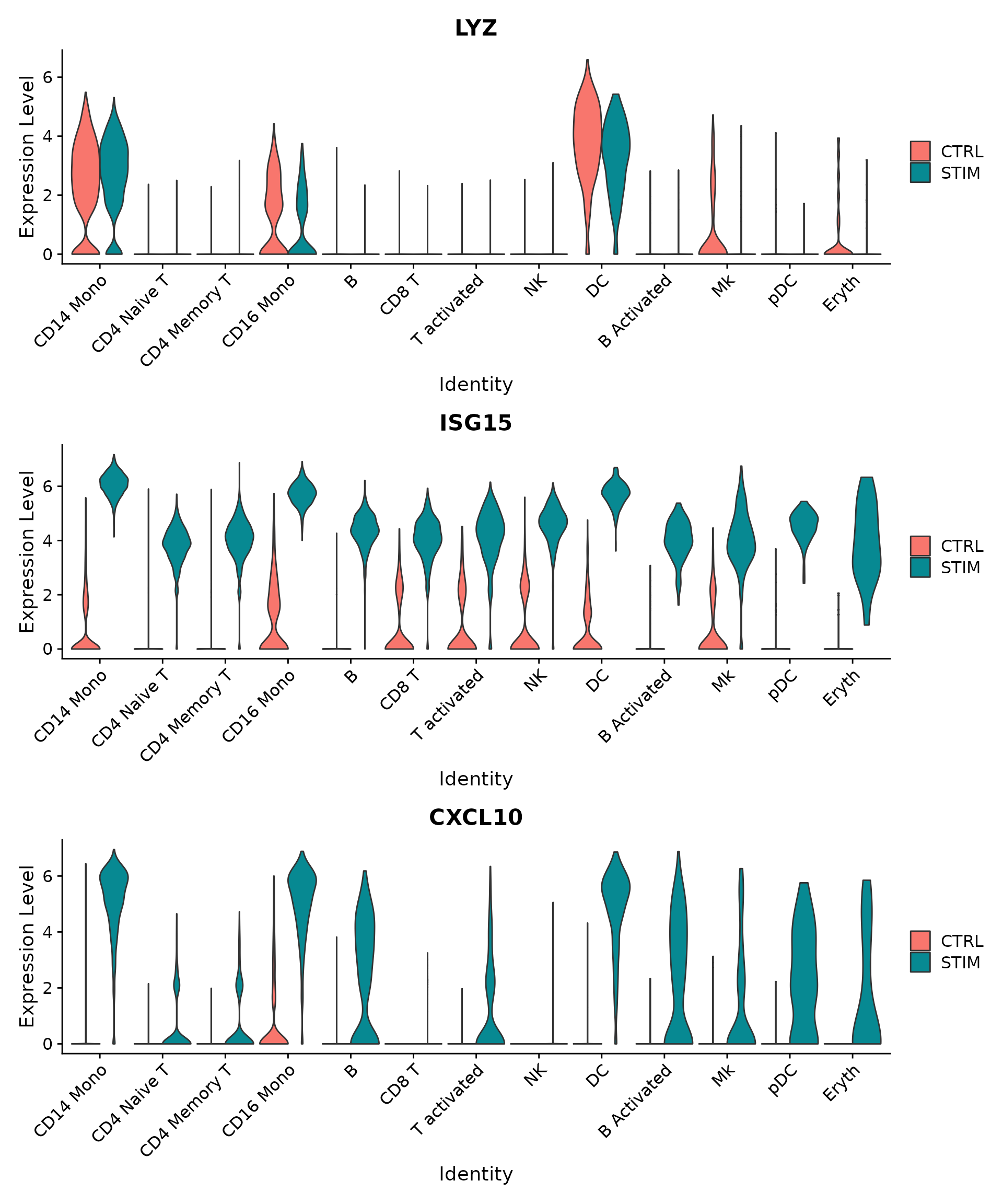
Perform integration with SCTransform-normalized datasets
As an alternative to log-normalization, Seurat also includes support
for preprocessing of scRNA-seq using the sctransform
workflow. The IntegrateLayers function also supports
SCTransform-normalized data, by setting the
normalization.method parameter, as shown below.
ifnb <- LoadData("ifnb")

# split datasets and process without integration
ifnb[["RNA"]] <- split(ifnb[["RNA"]], f = ifnb$stim)
ifnb <- SCTransform(ifnb)
ifnb <- RunPCA(ifnb)
ifnb <- RunUMAP(ifnb, dims = 1:30)
DimPlot(ifnb, reduction = "umap", group.by = c("stim", "seurat_annotations"))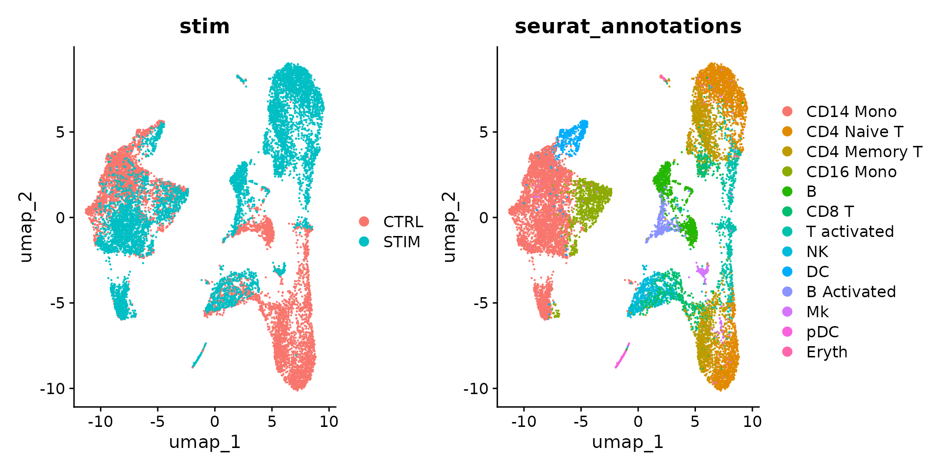
# integrate datasets
ifnb <- IntegrateLayers(object = ifnb, method = CCAIntegration, normalization.method = "SCT", verbose = F)
ifnb <- FindNeighbors(ifnb, reduction = "integrated.dr", dims = 1:30)
ifnb <- FindClusters(ifnb, resolution = 0.6)
## Modularity Optimizer version 1.3.0 by Ludo Waltman and Nees Jan van Eck
##
## Number of nodes: 13999
## Number of edges: 545244
##
## Running Louvain algorithm...
## Maximum modularity in 10 random starts: 0.9074
## Number of communities: 19
## Elapsed time: 2 seconds
ifnb <- RunUMAP(ifnb, dims = 1:30, reduction = "integrated.dr")
DimPlot(ifnb, reduction = "umap", group.by = c("stim", "seurat_annotations"))
# perform differential expression
ifnb <- PrepSCTFindMarkers(ifnb)
ifnb$celltype.stim <- paste(ifnb$seurat_annotations, ifnb$stim, sep = "_")
Idents(ifnb) <- "celltype.stim"
b.interferon.response <- FindMarkers(ifnb, ident.1 = "B_STIM", ident.2 = "B_CTRL", verbose = FALSE)
head(b.interferon.response, n = 15)
## p_val avg_log2FC pct.1 pct.2 p_val_adj
## ISG15 1.492226e-159 5.1598904 0.998 0.229 1.985556e-155
## IFIT3 4.131361e-154 6.2286235 0.961 0.052 5.497189e-150
## IFI6 2.479595e-153 5.6463400 0.965 0.076 3.299349e-149
## ISG20 9.385626e-152 3.1715979 1.000 0.666 1.248851e-147
## IFIT1 2.363477e-139 6.2629059 0.904 0.029 3.144843e-135
## MX1 2.111961e-124 4.1490465 0.900 0.115 2.810175e-120
## LY6E 2.930420e-122 3.9278136 0.898 0.150 3.899217e-118
## TNFSF10 1.104024e-112 6.8254288 0.785 0.020 1.469014e-108
## IFIT2 3.491368e-108 5.5668205 0.783 0.037 4.645615e-104
## B2M 3.323231e-98 0.6075636 1.000 1.000 4.421891e-94
## IRF7 1.114291e-96 3.3721350 0.834 0.187 1.482675e-92
## PLSCR1 3.364901e-96 4.0217697 0.783 0.111 4.477338e-92
## UBE2L6 1.155610e-85 2.6732717 0.849 0.295 1.537655e-81
## CXCL10 5.690116e-84 8.0934233 0.639 0.010 7.571268e-80
## PSMB9 2.304426e-81 1.8684260 0.937 0.568 3.066269e-77Session Info
## R version 4.5.2 (2025-10-31)
## Platform: x86_64-pc-linux-gnu
## Running under: Ubuntu 24.04.4 LTS
##
## Matrix products: default
## BLAS:   /usr/lib/x86_64-linux-gnu/openblas-pthread/libblas.so.3
## LAPACK: /usr/lib/x86_64-linux-gnu/openblas-pthread/libopenblasp-r0.3.26.so;  LAPACK version 3.12.0
##
## locale:
##  [1] LC_CTYPE=en_US.UTF-8       LC_NUMERIC=C
##  [3] LC_TIME=en_US.UTF-8        LC_COLLATE=en_US.UTF-8
##  [5] LC_MONETARY=en_US.UTF-8    LC_MESSAGES=en_US.UTF-8
##  [7] LC_PAPER=en_US.UTF-8       LC_NAME=C
##  [9] LC_ADDRESS=C               LC_TELEPHONE=C
## [11] LC_MEASUREMENT=en_US.UTF-8 LC_IDENTIFICATION=C
##
## time zone: Etc/UTC
## tzcode source: system (glibc)
##
## attached base packages:
## [1] stats     graphics  grDevices utils     datasets  methods   base
##
## other attached packages:
## [1] cowplot_1.2.0         ggplot2_4.0.3         future_1.70.0
## [4] patchwork_1.3.2       ifnb.SeuratData_3.1.0 SeuratData_0.2.2.9002
## [7] Seurat_5.5.0          SeuratObject_5.4.0    sp_2.2-1
##
## loaded via a namespace (and not attached):
##   [1] RcppAnnoy_0.0.23            splines_4.5.2
##   [3] later_1.4.8                 tibble_3.3.1
##   [5] polyclip_1.10-7             fastDummies_1.7.6
##   [7] lifecycle_1.0.5             Rdpack_2.6.6
##   [9] globals_0.19.1              lattice_0.22-7
##  [11] MASS_7.3-65                 magrittr_2.0.5
##  [13] limma_3.66.0                plotly_4.12.0
##  [15] sass_0.4.10                 rmarkdown_2.30
##  [17] jquerylib_0.1.4             yaml_2.3.12
##  [19] plotrix_3.8-14              qqconf_1.3.2
##  [21] httpuv_1.6.16               otel_0.2.0
##  [23] sn_2.1.3                    glmGamPoi_1.22.0
##  [25] sctransform_0.4.3           spam_2.11-3
##  [27] spatstat.sparse_3.1-0       reticulate_1.46.0
##  [29] pbapply_1.7-4               RColorBrewer_1.1-3
##  [31] multcomp_1.4-30             abind_1.4-8
##  [33] GenomicRanges_1.62.1        Rtsne_0.17
##  [35] purrr_1.2.1                 presto_1.0.0
##  [37] BiocGenerics_0.56.0         TH.data_1.1-5
##  [39] rappdirs_0.3.4              sandwich_3.1-1
##  [41] IRanges_2.44.0              S4Vectors_0.48.1
##  [43] ggrepel_0.9.8               irlba_2.3.7
##  [45] listenv_0.10.1              spatstat.utils_3.2-2
##  [47] TFisher_0.2.0               goftest_1.2-3
##  [49] RSpectra_0.16-2             spatstat.random_3.4-5
##  [51] fitdistrplus_1.2-6          parallelly_1.47.0
##  [53] DelayedMatrixStats_1.32.0   pkgdown_2.2.0
##  [55] DelayedArray_0.36.1         codetools_0.2-20
##  [57] tidyselect_1.2.1            farver_2.1.2
##  [59] matrixStats_1.5.0           stats4_4.5.2
##  [61] spatstat.explore_3.8-0      Seqinfo_1.0.0
##  [63] mathjaxr_2.0-0              jsonlite_2.0.0
##  [65] multtest_2.66.0             progressr_0.19.0
##  [67] ggridges_0.5.7              survival_3.8-3
##  [69] systemfonts_1.3.2           tools_4.5.2
##  [71] ragg_1.5.1                  ica_1.0-3
##  [73] Rcpp_1.1.1-1.1              glue_1.8.0
##  [75] SparseArray_1.10.10         mnormt_2.1.2
##  [77] gridExtra_2.3               xfun_0.56
##  [79] metap_1.13                  MatrixGenerics_1.22.0
##  [81] dplyr_1.2.0                 withr_3.0.2
##  [83] numDeriv_2016.8-1.1         formatR_1.14
##  [85] fastmap_1.2.0               digest_0.6.39
##  [87] R6_2.6.1                    mime_0.13
##  [89] textshaping_1.0.5           scattermore_1.2
##  [91] tensor_1.5.1                spatstat.data_3.1-9
##  [93] tidyr_1.3.2                 generics_0.1.4
##  [95] data.table_1.18.2.1         S4Arrays_1.10.1
##  [97] httr_1.4.8                  htmlwidgets_1.6.4
##  [99] uwot_0.2.4                  pkgconfig_2.0.3
## [101] gtable_0.3.6                lmtest_0.9-40
## [103] S7_0.2.1                    XVector_0.50.0
## [105] htmltools_0.5.9             dotCall64_1.2
## [107] scales_1.4.0                Biobase_2.70.0
## [109] png_0.1-9                   spatstat.univar_3.1-7
## [111] knitr_1.51                  reshape2_1.4.5
## [113] nlme_3.1-168                cachem_1.1.0
## [115] zoo_1.8-15                  stringr_1.6.0
## [117] KernSmooth_2.23-26          parallel_4.5.2
## [119] miniUI_0.1.2                vipor_0.4.7
## [121] ggrastr_1.0.2               desc_1.4.3
## [123] pillar_1.11.1               grid_4.5.2
## [125] vctrs_0.7.1                 RANN_2.6.2
## [127] promises_1.5.0              beachmat_2.26.0
## [129] xtable_1.8-8                cluster_2.1.8.2
## [131] beeswarm_0.4.0              evaluate_1.0.5
## [133] mvtnorm_1.3-7               cli_3.6.6
## [135] compiler_4.5.2              rlang_1.2.0
## [137] crayon_1.5.3                future.apply_1.20.2
## [139] mutoss_0.1-14               labeling_0.4.3
## [141] plyr_1.8.9                  fs_2.1.0
## [143] ggbeeswarm_0.7.3            stringi_1.8.7
## [145] viridisLite_0.4.3           deldir_2.0-4
## [147] lazyeval_0.2.3              spatstat.geom_3.7-3
## [149] Matrix_1.7-5                RcppHNSW_0.6.0
## [151] sparseMatrixStats_1.22.0    statmod_1.5.1
## [153] shiny_1.13.0                SummarizedExperiment_1.40.0
## [155] rbibutils_2.4.1             ROCR_1.0-12
## [157] igraph_2.3.0                bslib_0.10.0