Analysis, visualization, and integration of spatial datasets with Seurat
Compiled: May 27, 2026
Source:vignettes/spatial_vignette.Rmd
spatial_vignette.RmdOverview
This tutorial demonstrates how to use Seurat (>=3.2) to analyze spatially-resolved RNA-seq data. While the analysis pipelines are similar to the Seurat workflow for single-cell RNA-seq analysis, we introduce updated interaction and visualization tools, with a particular emphasis on the integration of spatial and molecular information. This tutorial will cover the following tasks, which we believe will be common for many spatial analyses:
- Normalization
- Dimensional reduction and clustering
- Detecting spatially-variable features
- Interactive visualization
- Integration with single-cell RNA-seq data
- Working with multiple slices
Here we show the analysis of spatial datasets generated with the 1) Visium platform from 10x Genomics and 2) SLIDE-seq from the Macosko Lab.
For related vignettes, please see the Spatial Analysis section of the vignette landing page.
10x Visium
Dataset
We will be using a dataset of sagittal mouse brain slices generated using the Visium v1 chemistry. There are two serial anterior sections and two (matched) serial posterior sections.
You can download the data from 10x Genomics’ dataset repository (Sagittal-Anterior Section 1, Section 2; Sagittal-Posterior Section 1, Section 2) and load it into Seurat using the Load10X_Spatial() function. This reads in the output of the Space Ranger count pipeline, and returns a Seurat object that contains both the spot-level expression data along with the associated image of the tissue slice.
You can also use our SeuratData
package for easy data access, as demonstrated below. After
installing the dataset, you can type ?stxBrain to learn
more.
InstallData("stxBrain")
brain <- LoadData("stxBrain", type = "anterior1")How is the spatial data stored within Seurat?
The visium data from 10x consists of the following data types:
- A spot by gene expression matrix
- An image of the tissue slice (obtained from H&E staining during data acquisition)
- Scale factors that relate the original high-resolution image to the lower resolution image used for visualization
Assay but contains spot level, not
single-cell level data. The image itself is stored in a new
images slot in the Seurat object. The images
slot also stores the information necessary to associate spots with their
physical position on the tissue image.
Data preprocessing
The initial preprocessing steps that we perform on the spot-by-gene expression data are similar to a typical scRNA-seq experiment. We first need to normalize the data in order to account for variance in sequencing depth across data points. We note that the variance in molecular counts / spot can be substantial for spatial datasets, particularly if there are differences in cell density across the tissue. We see substantial heterogeneity here, which requires effective normalization.
plot1 <- VlnPlot(brain, features = "nCount_Spatial", pt.size = 0.1) + NoLegend()

plot2 <- SpatialFeaturePlot(brain, features = "nCount_Spatial") + theme(legend.position = "right")

wrap_plots(plot1, plot2)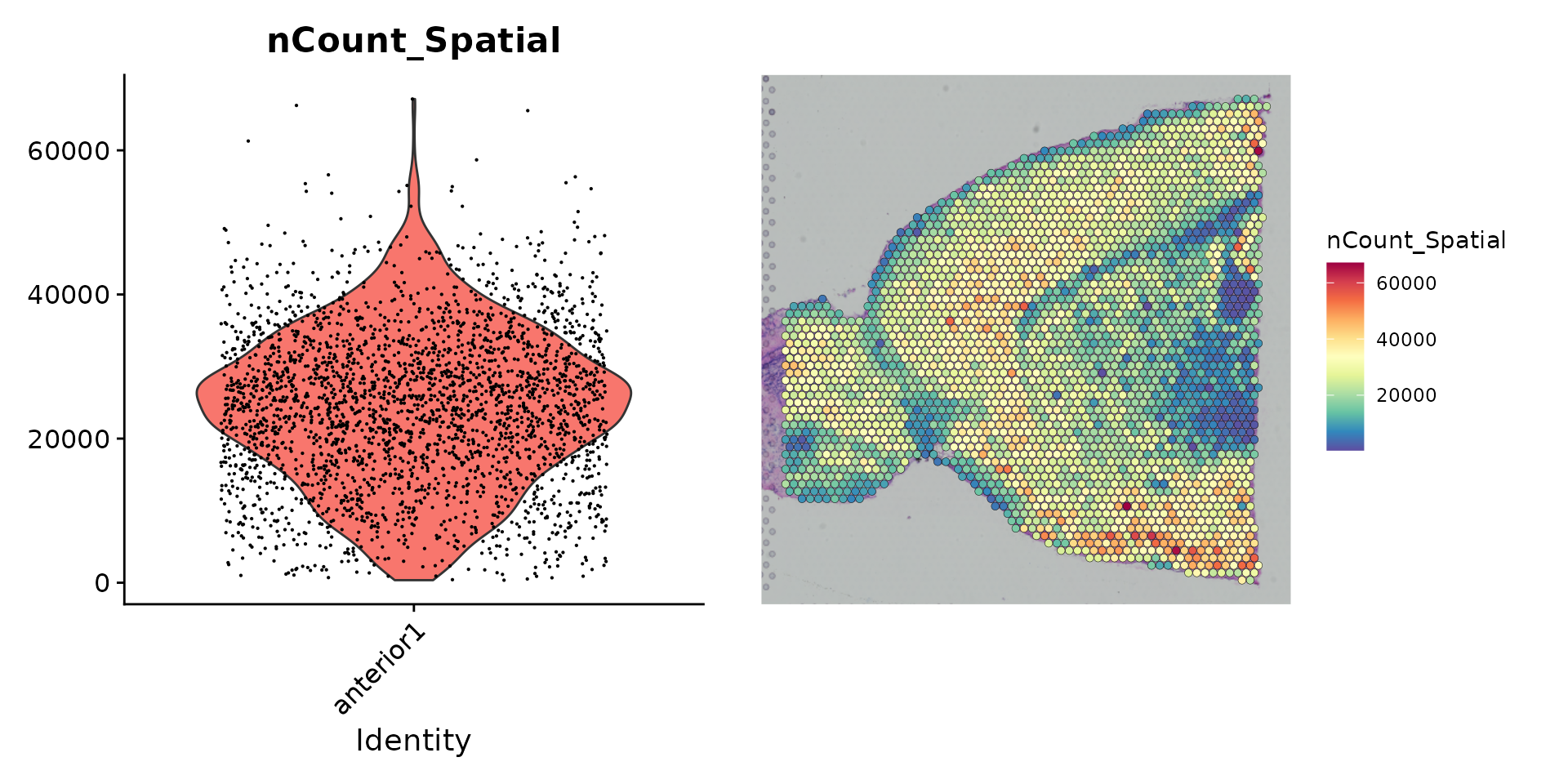
These plots demonstrate that the variance in molecular counts across spots is not just technical in nature, but is also dependent on the tissue anatomy. In this vignette, we proceed with using sctransform (Hafemeister and Satija, Genome Biology 2019) for normalization, which builds regularized negative binomial models of gene expression in order to account for technical artifacts while preserving biological variance. However, we emphasize that the best normalization methods for spatial data are still being developed and evaluated, and encourage users to read manuscripts from the Phipson/Davis and Fan labs to learn more about potential caveats for spatial normalization.
brain <- SCTransform(brain, assay = "Spatial", verbose = FALSE)Gene expression visualization
In Seurat, we have functionality to explore and interact with the
inherently visual nature of spatial data. The
SpatialFeaturePlot() function in Seurat extends
FeaturePlot(), and can overlay molecular data on top of
tissue histology. For example, in this data set of the mouse brain, the
gene Hpca is a strong hippocampus marker and Ttr is a
marker of the choroid plexus.
SpatialFeaturePlot(brain, features = c("Hpca", "Ttr"))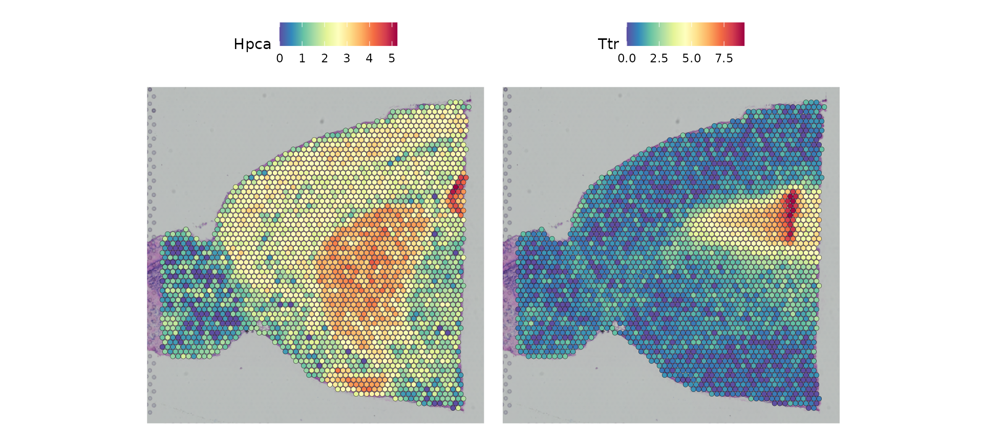
As with other visualization functions in Seurat, the spatial plotting
functions return ggplot2 objects, so additional layers can
be added for customization, as below.
custom_plot <- SpatialFeaturePlot(brain, features = c("Ttr")) +
                theme(legend.text = element_text(size = 0),
                      legend.title = element_text(size = 20),
                      legend.key.size = unit(1, "cm"))

custom_plot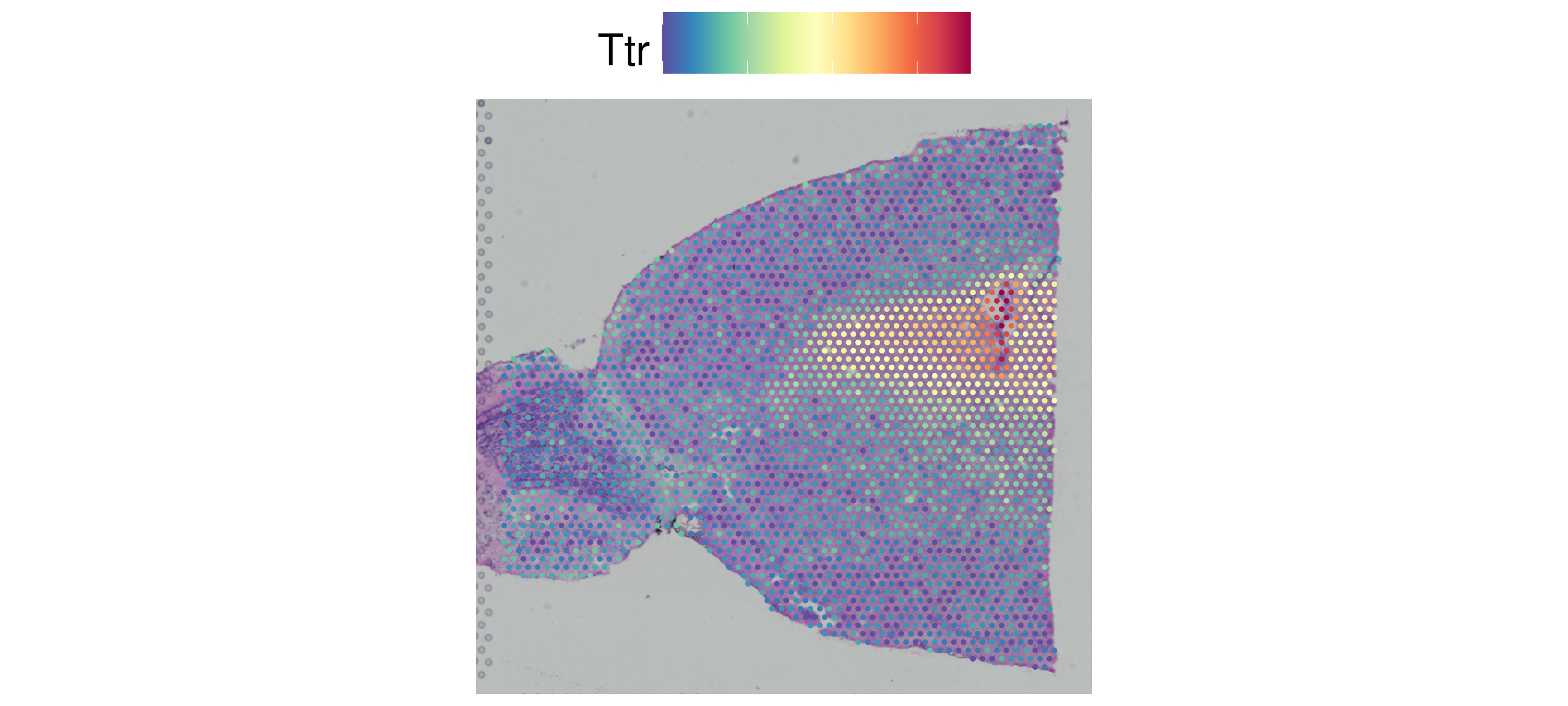
The default parameters in Seurat emphasize the visualization of molecular data. Users can also adjust the size of the spots (and their transparency) to improve the visualization of the histology image, by changing different parameters. We encourage users to explore these options through the function documentation.
For example, below, we try a different scale factor for point size
and set alpha = c(0.1, 1), to downweight the transparency
of points with lower expression.
p1 <- SpatialFeaturePlot(brain, features = "Ttr", pt.size.factor = 1)

p2 <- SpatialFeaturePlot(brain, features = "Ttr", alpha = c(0.1, 1))

p1 + p2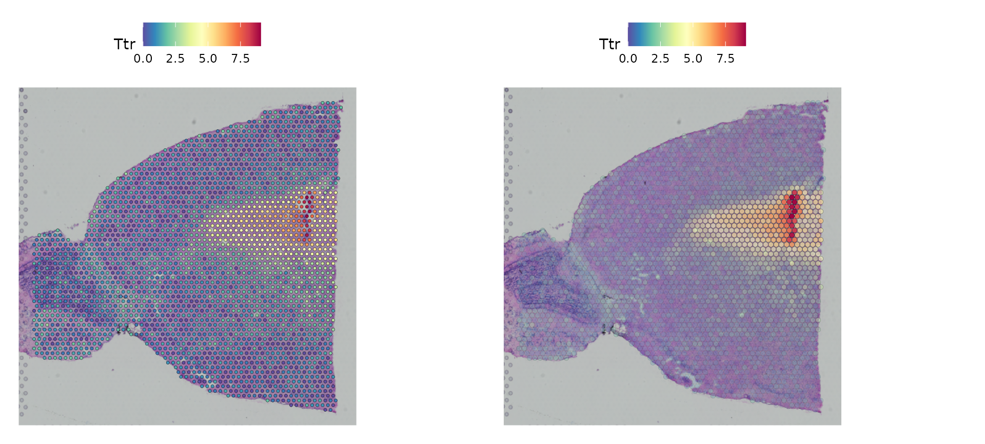
Dimensionality reduction, clustering, and visualization
We can then proceed to run dimensionality reduction and clustering on the RNA expression data, using the same workflow as we use for scRNA-seq analysis.
brain <- RunPCA(brain, assay = "SCT", verbose = FALSE)
brain <- FindNeighbors(brain, reduction = "pca", dims = 1:30)
brain <- FindClusters(brain, verbose = FALSE)
brain <- RunUMAP(brain, reduction = "pca", dims = 1:30)
We can then visualize the results of the clustering either in UMAP
space (with DimPlot()) or overlaid on the image with
SpatialDimPlot().
p1 <- DimPlot(brain, reduction = "umap", label = TRUE)

p2 <- SpatialDimPlot(brain, label = TRUE, label.size = 3)

p1 + p2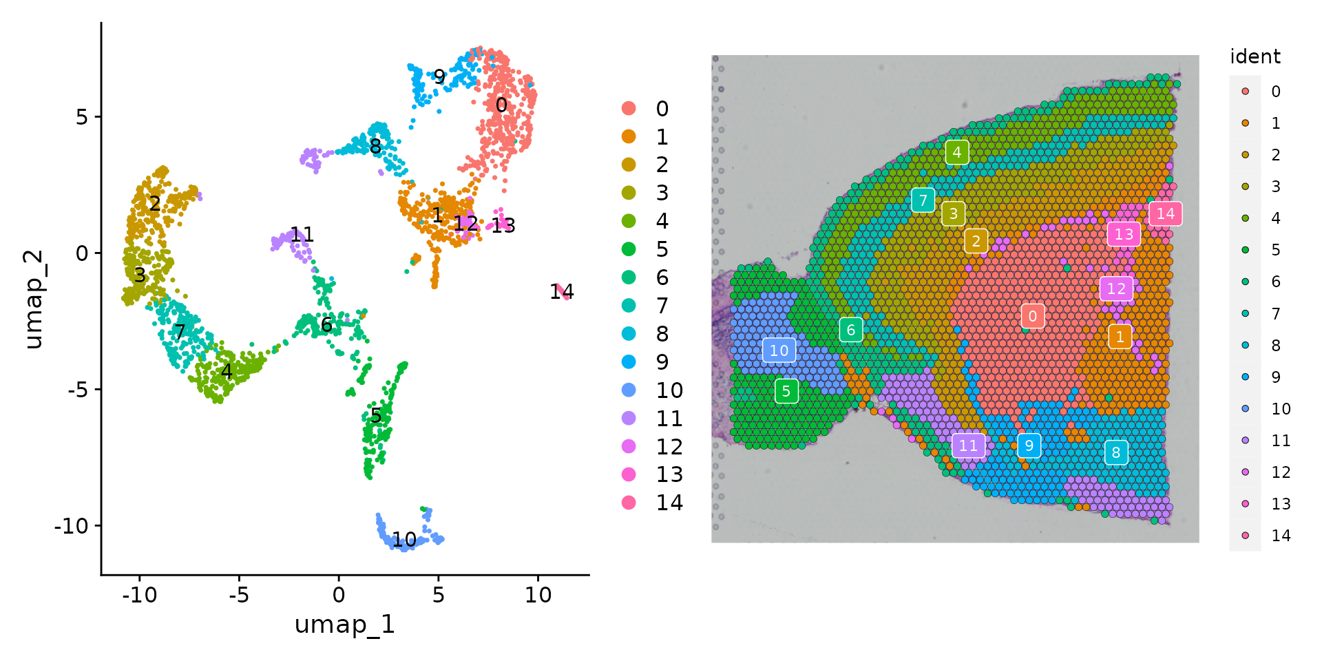
As there are many colors, it can be challenging to visualize which
voxel belongs to which cluster. We have a few strategies to help with
this. Setting the label parameter places a colored box at
the median of each cluster (as in the plot above).
You can also use the cells.highlight parameter to
demarcate particular cells of interest on a
SpatialDimPlot(). This can be very useful for
distinguishing the spatial localization of individual clusters:
SpatialDimPlot(brain,
               cells.highlight = CellsByIdentities(object = brain, idents = c(2, 1, 4, 3, 5, 8)),
               facet.highlight = TRUE,
               ncol = 3) & theme(plot.margin = unit(c(1, 1, 1, 1), "mm"))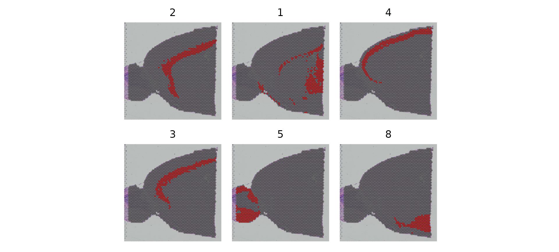
Interactive plotting
We have also built in a number of interactive plotting capabilities.
Both SpatialDimPlot() and SpatialFeaturePlot()
have an interactive parameter, that when set to TRUE, open
an interactive Shiny environment. Users can explore the data
interactively and afterwards select “Done” to return the last active
plot as a ggplot2 object.
The example below demonstrates an
interactive SpatialDimPlot() in which hovering over spots
shows the cell name and current identity class (analogous to the
previous do.hover behavior).
SpatialDimPlot(brain, interactive = TRUE)For SpatialFeaturePlot(), setting
interactive to TRUE allows for adjusting the
transparency of the spots, the point size, as well as the Assay and
feature being plotted.
SpatialFeaturePlot(brain, features = "Ttr", interactive = TRUE)LinkedDimPlot() links the UMAP representation to the
tissue image representation and allows for interactive selection. For
example, you can select a region in the UMAP plot and the corresponding
spots in the image representation will be highlighted.
LinkedDimPlot(brain)Identification of Spatially Variable Features
Seurat offers two workflows to identify molecular features that correlate with spatial location within a tissue. The first is to perform differential expression based on pre-annotated anatomical regions within the tissue, which may be determined either from unsupervised clustering or prior knowledge. This strategy works will in this case, as the clusters above exhibit clear spatial restriction.
de_markers <- FindMarkers(brain, ident.1 = 5, ident.2 = 7)

SpatialFeaturePlot(object = brain, features = rownames(de_markers)[1:3], alpha = c(0.1, 1), ncol = 3)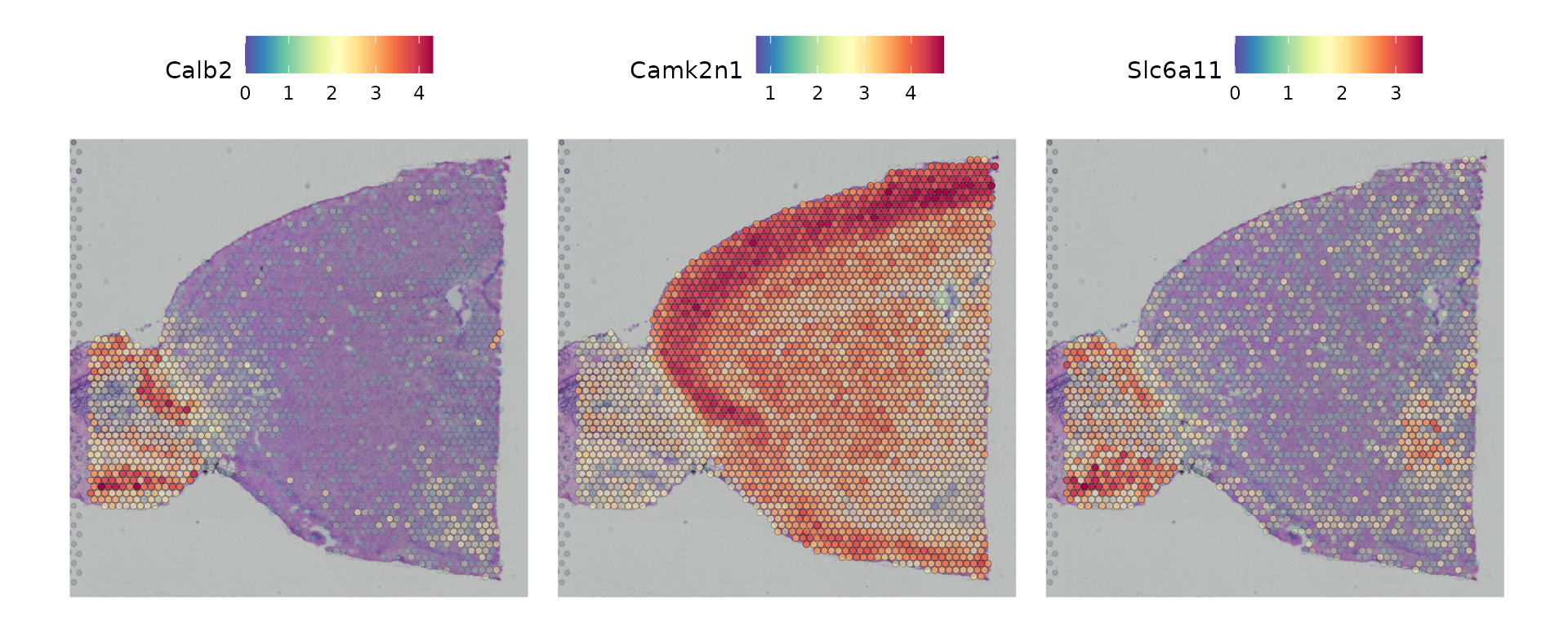
An alternative approach, implemented in
FindSpatiallyVariableFeatures(), is to search for features
exhibiting spatial patterning in the absence of pre-annotation. One of
the default methods, (selection.method = "markvariogram"),
is inspired by trendsceek,
which models ST data as a mark point process and computes a ‘variogram’,
identifying genes whose expression level is dependent on their spatial
location.1 Here, we specify
selection.method = "moransi", which uses Moran’s I as a
spatial autocorrelation metric.
We note that there are multiple methods in the literature to accomplish this task, including SpatialDE and Splotch. We encourage interested users to explore these methods as well, and hope to add support for them in the near future.
brain <- FindSpatiallyVariableFeatures(brain,
                                       features = VariableFeatures(brain)[1:1000],
                                       selection.method = "moransi")
Now we visualize the expression of the top 6 features identified by this measure.
top.features <- head(SpatiallyVariableFeatures(brain, method = "moransi"), 6)

SpatialFeaturePlot(brain, features = top.features, ncol = 3, alpha = c(0.1, 1)) &
  theme(plot.margin = unit(c(1, 1, 1, 1), "mm"))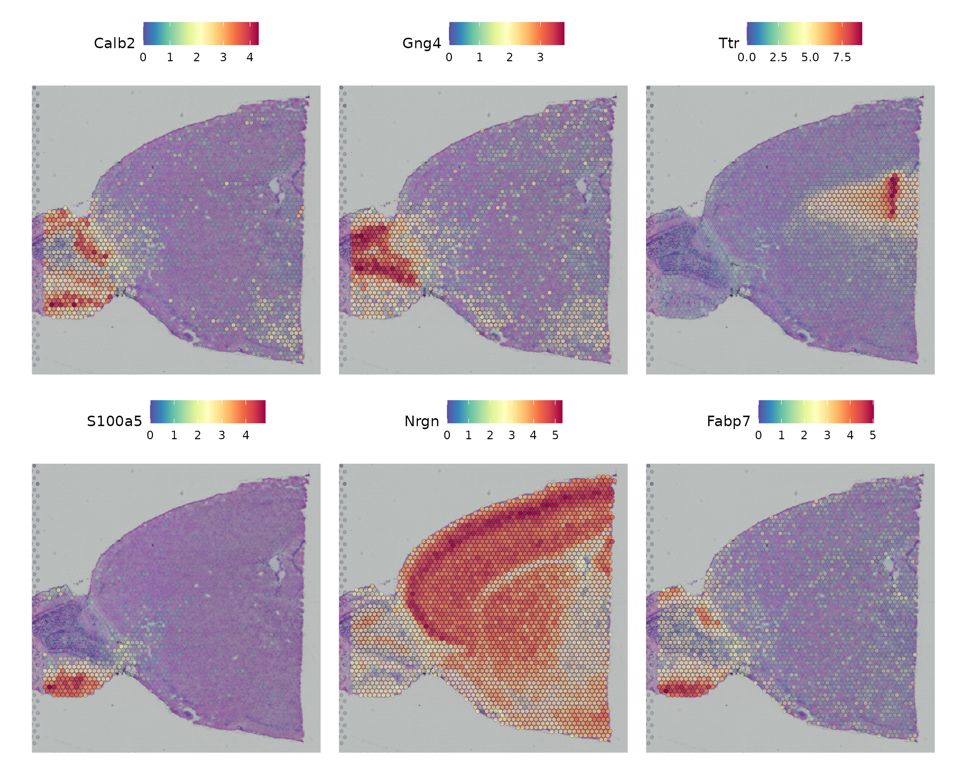
Subset out anatomical regions
Here, we approximately subset the frontal cortex. This process also facilitates the integration of these data with a cortical scRNA-seq dataset in the next section. First, we take a subset of clusters, and then further segment based on exact positions. After subsetting, we can visualize the cortical cells either on the full image, or a cropped image.
First, we subset by cluster:
brain_sub <- subset(brain, idents = c(1, 2, 3, 4, 6, 7))
SpatialDimPlot(brain_sub, label = T, crop = T, label.size = 3) + NoLegend() +
SpatialDimPlot(brain_sub, label = T, crop = F, label.size = 3)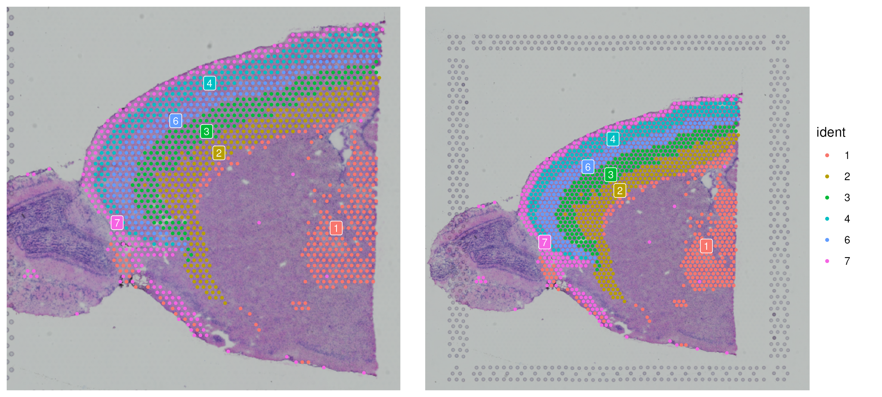 Now we can examine approximately which region to subset to by plotting
with the axes labeled:
Now we can examine approximately which region to subset to by plotting
with the axes labeled:
theme_axis_labels <- theme(axis.text.x = element_text(size = 10),
axis.text.y = element_text(size = 10),
axis.title.x = element_text(size = 10),
axis.title.y = element_text(size = 10))
SpatialDimPlot(brain_sub, label = T, label.size = 3, crop = T) + theme_axis_labels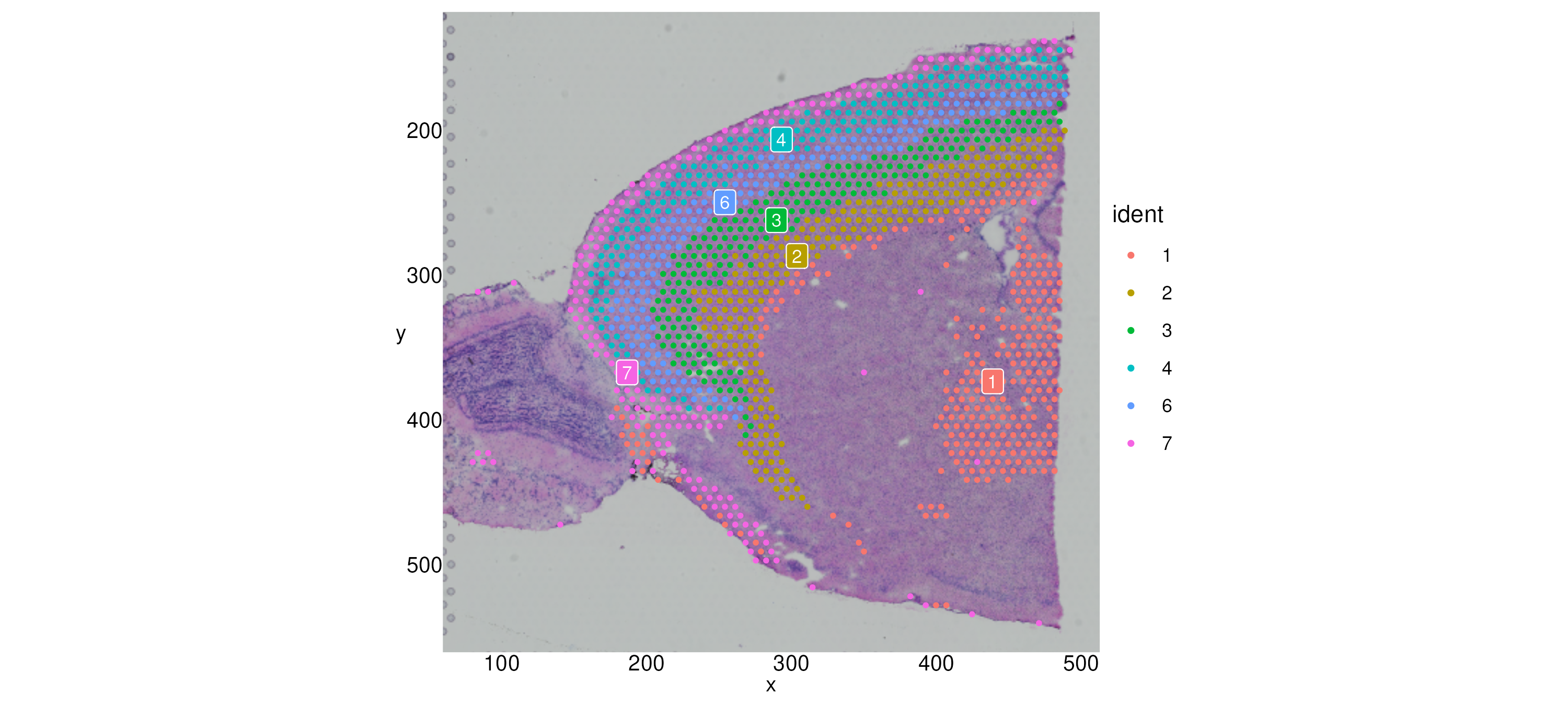 We can zoom in to a particular region with
 Crop():
brain_sub[["anterior1"]] <- Crop(brain_sub[["anterior1"]],
x = c(150, 500),
y = c(0, 425))
SpatialDimPlot(brain_sub, label = T) + theme_axis_labels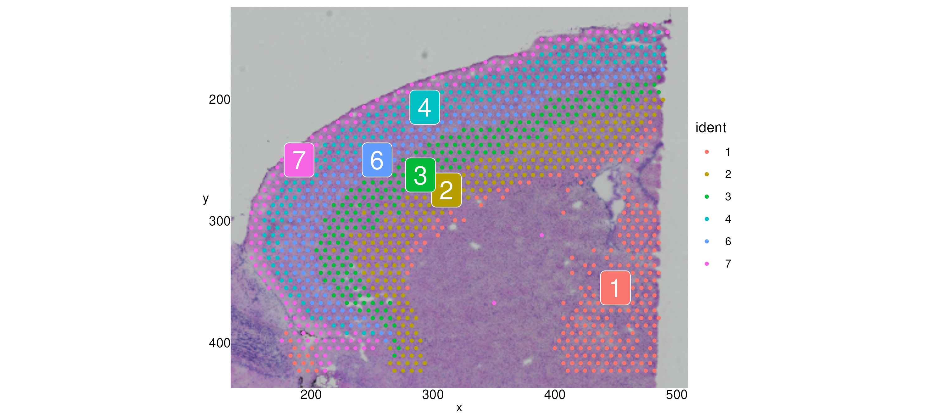 Finally, we subset out the cells in the lower right quadrant. Note that
because our coordinates are in image space, we need to be careful when
subsetting using a line—the y-coordinates in Cartesian space are
negative, since the direction of our y-axis is downward.
Finally, we subset out the cells in the lower right quadrant. Note that
because our coordinates are in image space, we need to be careful when
subsetting using a line—the y-coordinates in Cartesian space are
negative, since the direction of our y-axis is downward.
m <- 0.6; b <- -550

cortex_coords <- GetTissueCoordinates(brain_sub, scale = "lowres") %>%
                  subset(-y >= (m * x + b))

cortex <- subset(brain_sub,
                 cells = cortex_coords$cell)
SpatialDimPlot(cortex, label = T, label.size = 3, crop = F)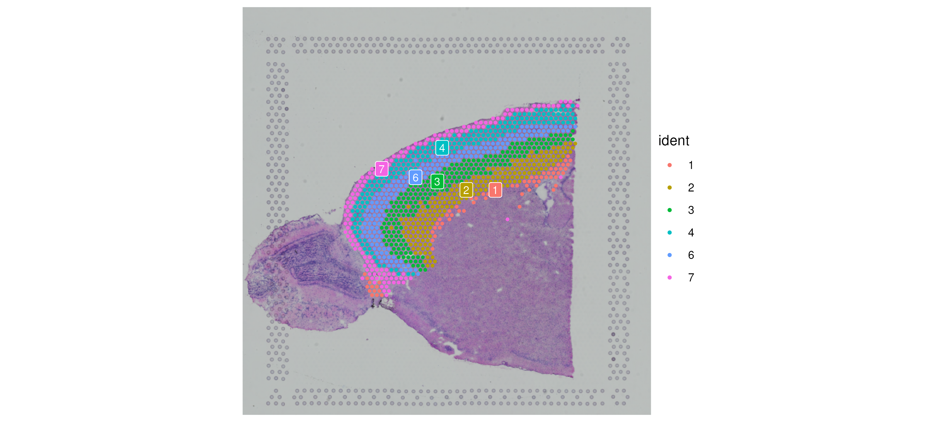
c1 <- SpatialDimPlot(cortex, images = "anterior1", crop = T, label = T)
c2 <- SpatialDimPlot(cortex, images = "anterior1", crop = F, label = T, pt.size.factor = 1, label.size = 3)

c1 + c2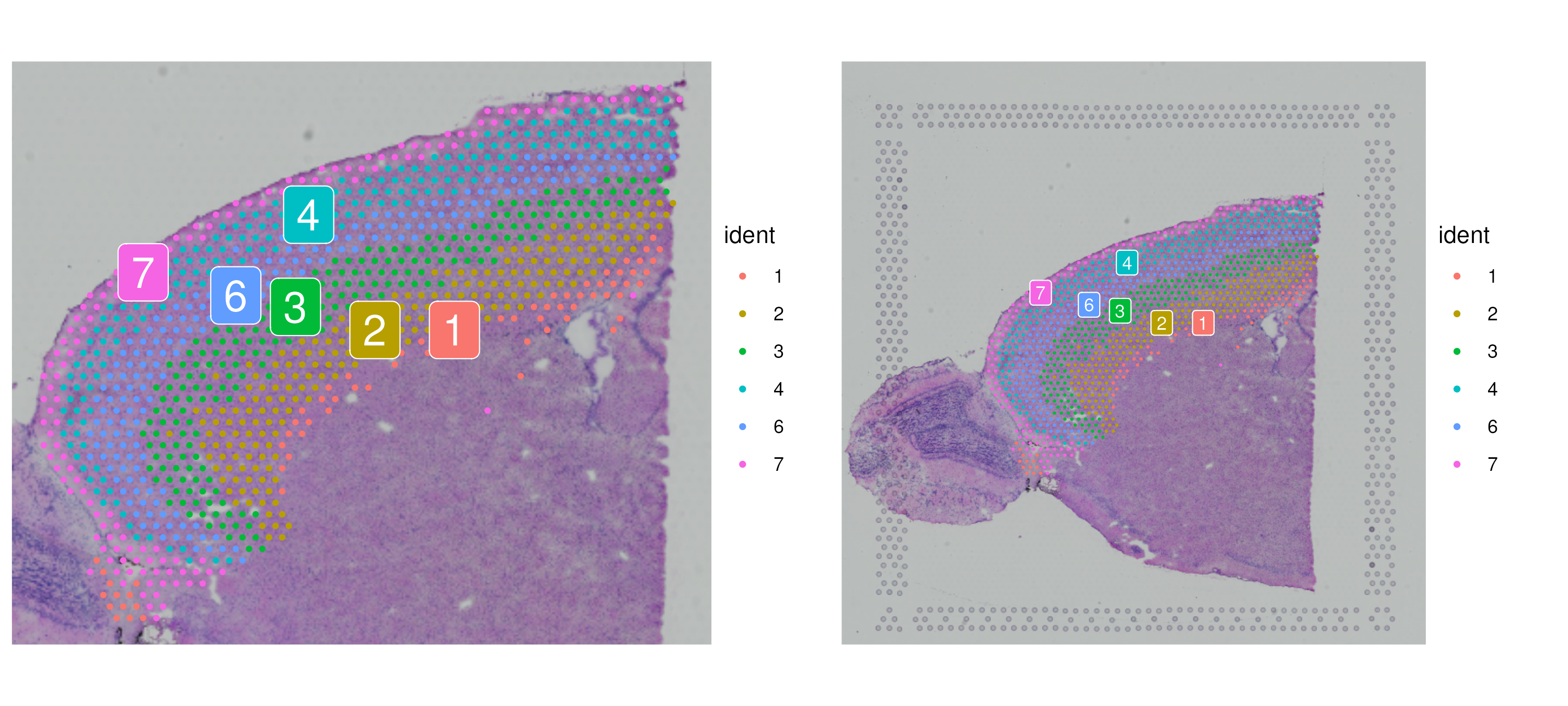
Integration with single-cell data
At ~50um, spots from the Visium assay will encompass the expression profiles of multiple cells. For the growing list of systems where scRNA-seq data is available, users may be interested to ‘deconvolute’ each of the spatial voxels to predict the underlying composition of cell types. In preparing this vignette, we tested a wide variety of deconvolution and integration methods, using a reference scRNA-seq dataset of ~14,000 adult mouse cortical cell taxonomy from the Allen Institute, generated with the SMART-Seq2 protocol.
We consistently found superior performance using integration methods (as opposed to deconvolution methods), likely because of substantially different noise models that characterize spatial and single-cell datasets, and integration methods are specifically designed to be robust to these differences. We therefore apply the ‘anchor’-based integration workflow introduced in Seurat v3, that enables the probabilistic transfer of annotations from a reference to a query set. We follow the label transfer workflow introduced here, taking advantage of sctransform normalization, but anticipate new methods to be developed to accomplish this task.
We first load the data (download available here), pre-process the scRNA-seq reference, and then perform label transfer. The procedure outputs, for each spot, a probabilistic classification for each of the scRNA-seq derived classes. We add these predictions as a new assay in the Seurat object.
allen_reference <- readRDS("/brahms/shared/vignette-data/allen_cortex.rds")
# Note: setting ncells=3000 normalizes the full dataset, but learns noise models on 3k cells
# This speeds up SCTransform dramatically with no loss in performance
allen_reference <- SCTransform(allen_reference, ncells = 3000, verbose = FALSE) %>%
                      RunPCA(verbose = FALSE) %>%
                      RunUMAP(dims = 1:30)
# The annotation is stored in the 'subclass' column of object metadata
DimPlot(allen_reference, group.by = "subclass", label = TRUE)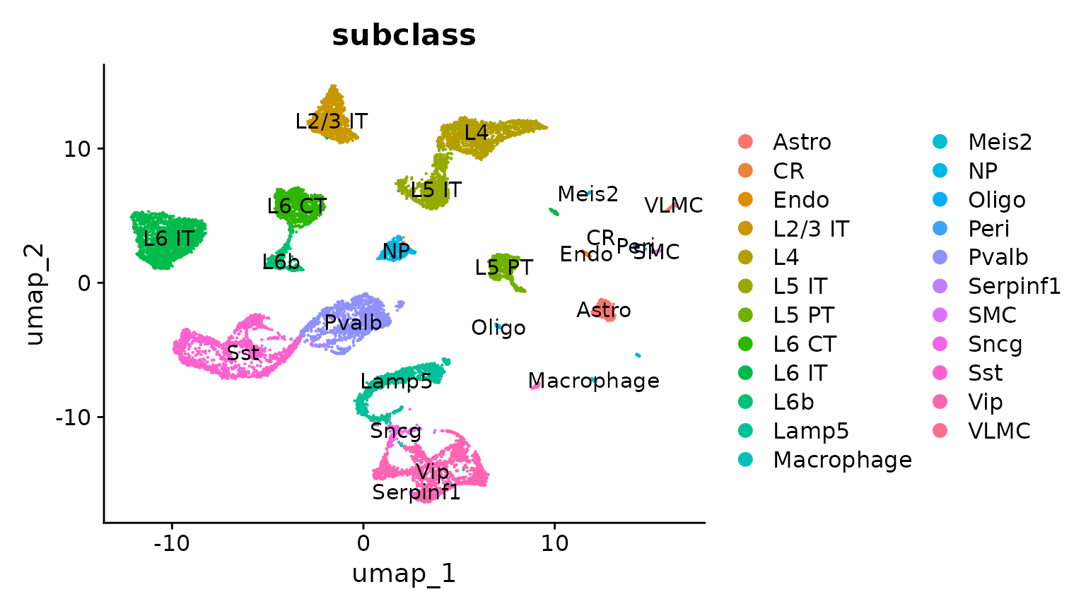
anchors <- FindTransferAnchors(reference = allen_reference,
                               query = cortex)

predictions.assay <- TransferData(anchorset = anchors,
                                  refdata = allen_reference$subclass,
                                  prediction.assay = TRUE,
                                  weight.reduction = cortex[["pca"]],
                                  dims = 1:30)

cortex[["predictions"]] <- predictions.assay
Now we get prediction scores for each spot for each class. Of particular interest in the frontal cortex region are the laminar excitatory neurons. Here we can distinguish between distinct sequential layers of these neuronal subtypes; for example:
DefaultAssay(cortex) <- "predictions"

SpatialFeaturePlot(cortex, features = c("L2/3 IT", "L4"), ncol = 2, crop = TRUE) &
  theme(plot.margin = unit(c(1, 1, 1, 1), "mm"))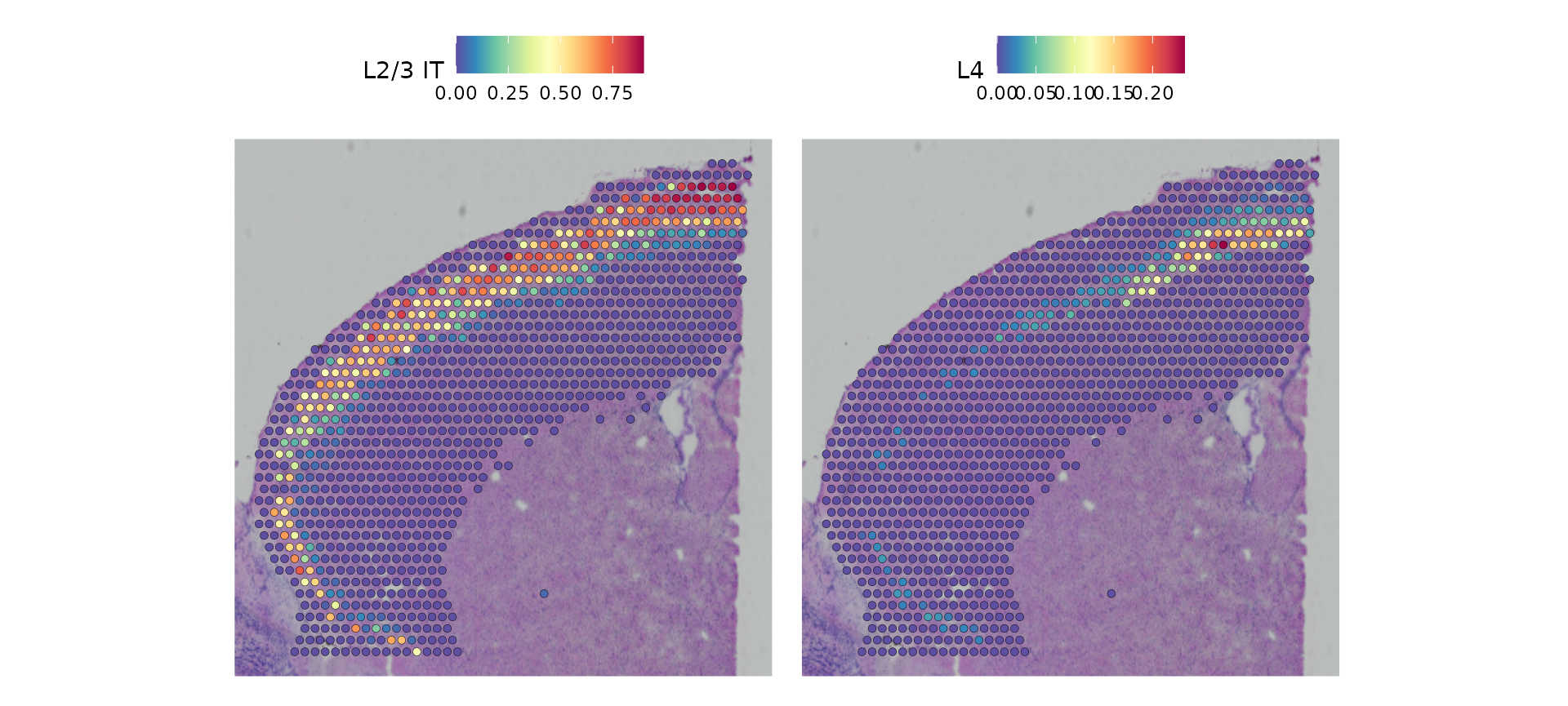
Based on these prediction scores, we can also predict cell types whose location is spatially restricted. We use the same methods based on marked point processes to define spatially variable features, but use the cell type prediction scores as the “marks” rather than gene expression.
cortex <- FindSpatiallyVariableFeatures(cortex,
                                        assay = "predictions",
                                        selection.method = "moransi",
                                        features = rownames(cortex),
                                        r.metric = 5,
                                        layer = "data")

top.clusters <- head(SpatiallyVariableFeatures(cortex, method = "moransi"), 4)

SpatialFeaturePlot(object = cortex, features = top.clusters, ncol = 2) &
  theme(plot.margin = unit(c(1, 1, 1, 1), "mm"))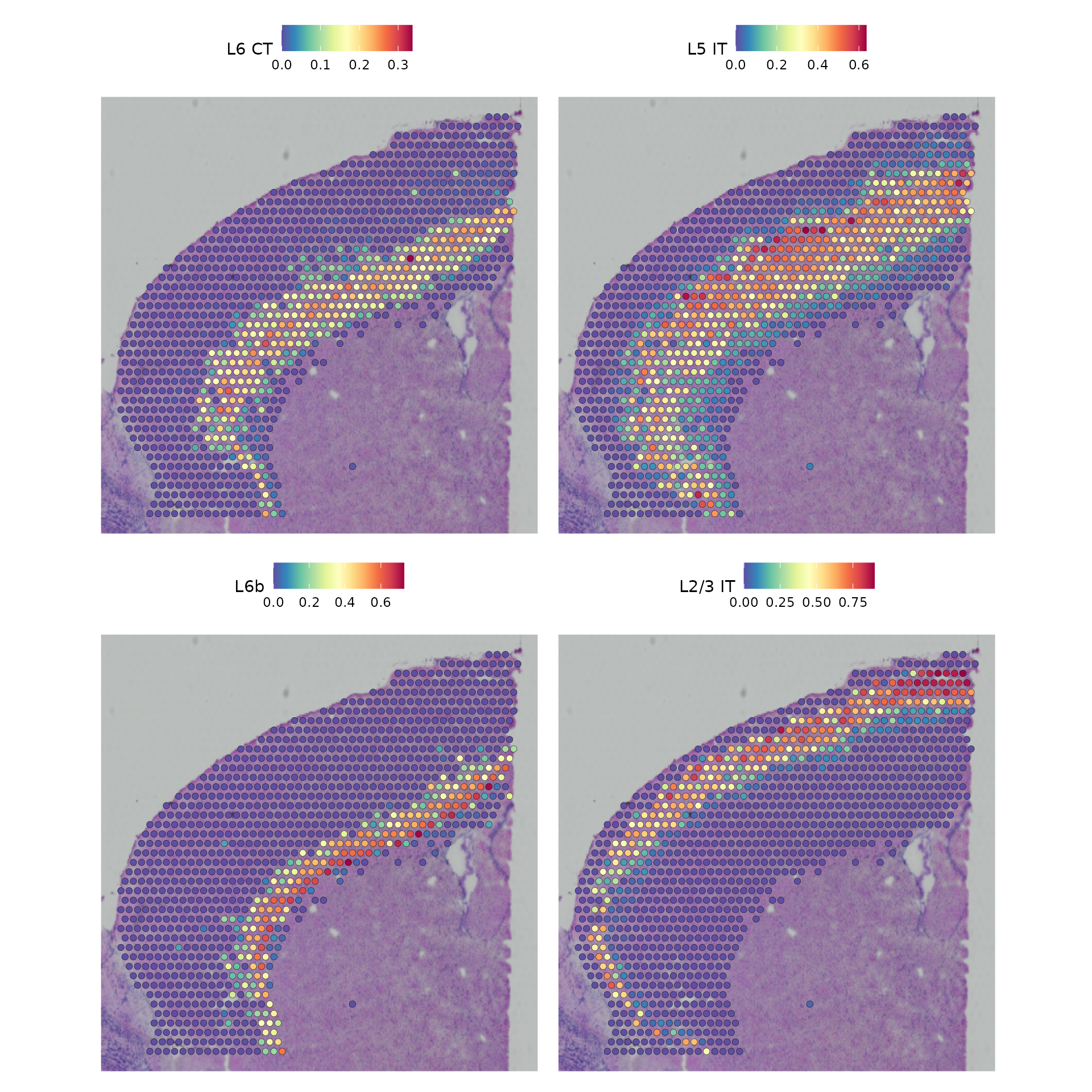
Finally, we show that our integrative procedure is capable of recovering the known spatial localization patterns of both neuronal and non-neuronal subsets, including laminar excitatory, layer-1 astrocytes, and the cortical grey matter.
features_of_interest <- c("Astro", "L2/3 IT", "L4", "L5 PT", "L5 IT", "L6 CT", "L6 IT", "L6b", "Oligo")

SpatialFeaturePlot(cortex,
                   features = features_of_interest,
                   pt.size.factor = 1,
                   ncol = 2,
                   crop = TRUE,
                   alpha = c(0.1, 1)) & theme(plot.margin = unit(c(1, 1, 1, 1), "mm")) &
                theme(plot.margin = unit(c(1, 1, 1, 1), "mm"))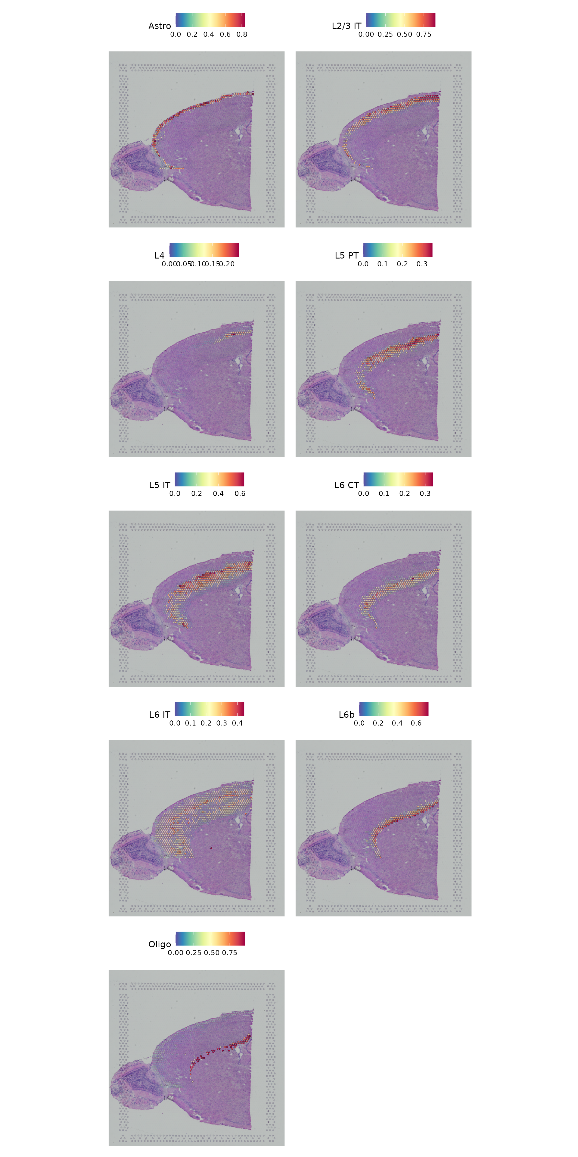
Working with multiple slices
This dataset of the mouse brain contains another slice corresponding to the other half of the brain. Here we read it in and perform the same initial normalization.
brain2 <- LoadData("stxBrain", type = "posterior1")

brain2 <- SCTransform(brain2, assay = "Spatial", verbose = FALSE)
In order to work with multiple slices in the same Seurat object, we
provide the merge function.
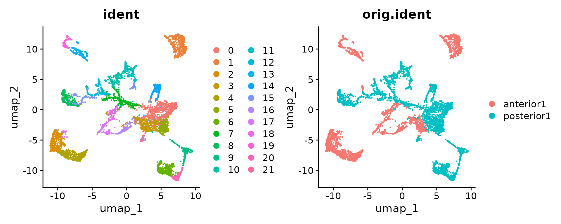
brain.merge <- merge(brain, brain2)This then enables joint dimensional reduction and clustering on the underlying RNA expression data.
DefaultAssay(brain.merge) <- "SCT"
VariableFeatures(brain.merge) <- c(VariableFeatures(brain), VariableFeatures(brain2))
brain.merge <- RunPCA(brain.merge, verbose = FALSE)
brain.merge <- FindNeighbors(brain.merge, dims = 1:30)
brain.merge <- FindClusters(brain.merge, verbose = FALSE)
brain.merge <- RunUMAP(brain.merge, dims = 1:30)
Finally, the data can be jointly visualized in a single UMAP plot.
SpatialDimPlot() and SpatialFeaturePlot() will
by default plot all slices as columns and groupings/features as
rows.
SpatialDimPlot(brain.merge)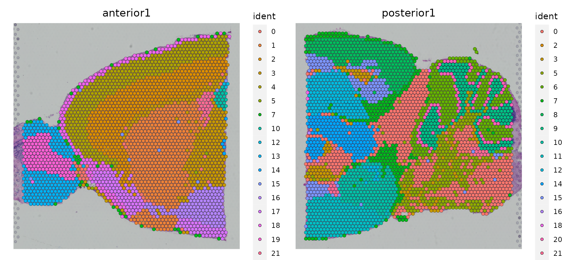
SpatialFeaturePlot(brain.merge, features = c("Hpca", "Plp1"))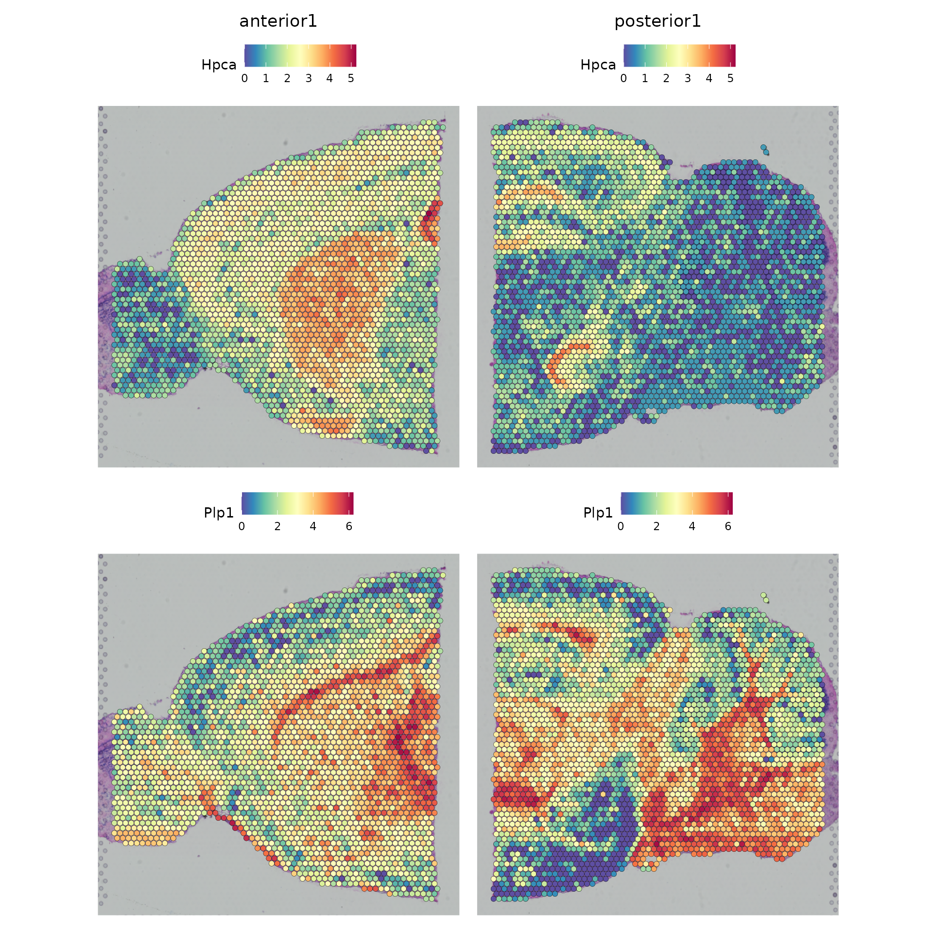
Slide-seq
Dataset
Here, we will be analyzing a dataset generated using Slide-seq v2 of the mouse hippocampus. This tutorial will follow much of the same structure as the tutorial for 10x Visium data above, but is tailored to give a demonstration specific to Slide-seq data.
You can use our SeuratData package for easy data access, as demonstrated below. After installing the dataset, you can type ?ssHippo to see the commands used to create the Seurat object.
InstallData("ssHippo")
slide.seq <- LoadData('ssHippo')Data preprocessing
The initial preprocessing steps for the bead by gene expression data are similar to other spatial Seurat analyses and to typical scRNA-seq experiments. Here, we note that many beads contain particularly low UMI counts, but choose to keep all detected beads for downstream analysis.
plot1 <- VlnPlot(slide.seq, features = 'nCount_Spatial', pt.size = 0, log = TRUE) + NoLegend()
slide.seq$log_nCount_Spatial <- log(slide.seq$nCount_Spatial)
plot2 <- SpatialFeaturePlot(slide.seq, features = 'log_nCount_Spatial') + theme(legend.position = "right")
wrap_plots(plot1, plot2)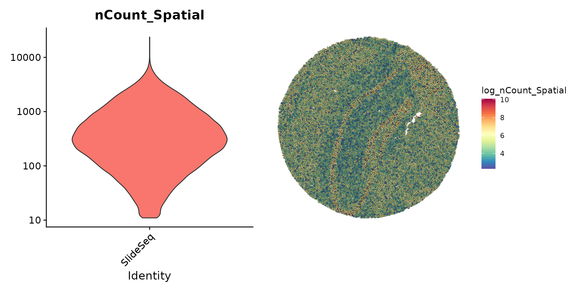
We then normalize the data using sctransform and perform a standard scRNA-seq dimensionality reduction and clustering workflow.
slide.seq <- SCTransform(slide.seq, assay = "Spatial", ncells = 3000, verbose = FALSE)
slide.seq <- RunPCA(slide.seq)
slide.seq <- RunUMAP(slide.seq, dims = 1:30)
slide.seq <- FindNeighbors(slide.seq, dims = 1:30)
slide.seq <- FindClusters(slide.seq, resolution = 0.3, verbose = FALSE)
We can then visualize the results of the clustering either in UMAP
space (with DimPlot()) or in the bead coordinate space with
SpatialDimPlot().
plot1 <- DimPlot(slide.seq, reduction = "umap", label = TRUE)
plot2 <- SpatialDimPlot(slide.seq, stroke = 0)
plot1 + plot2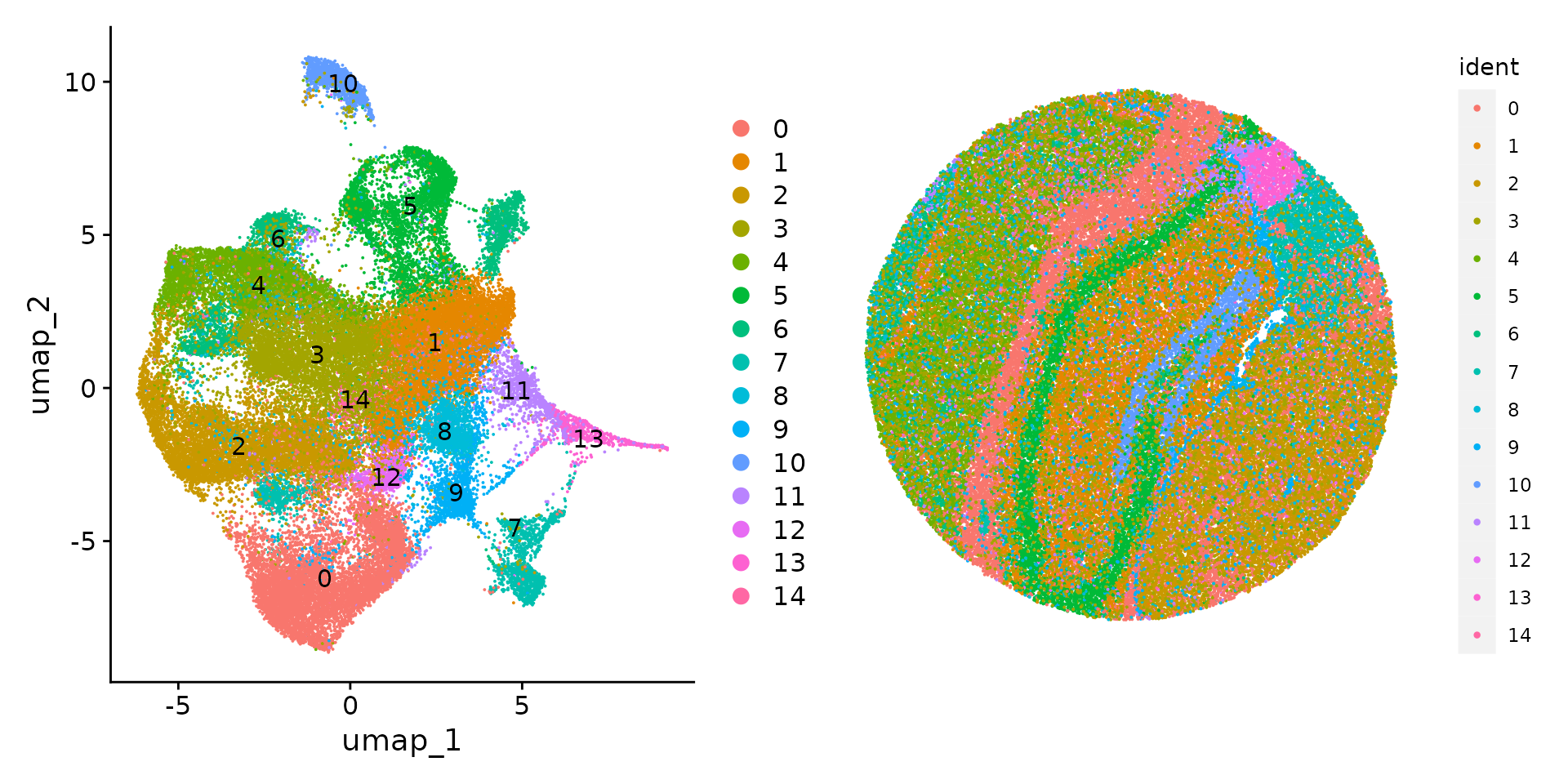
SpatialDimPlot(slide.seq, cells.highlight = CellsByIdentities(object = slide.seq, idents = c(1, 6, 13)), facet.highlight = TRUE)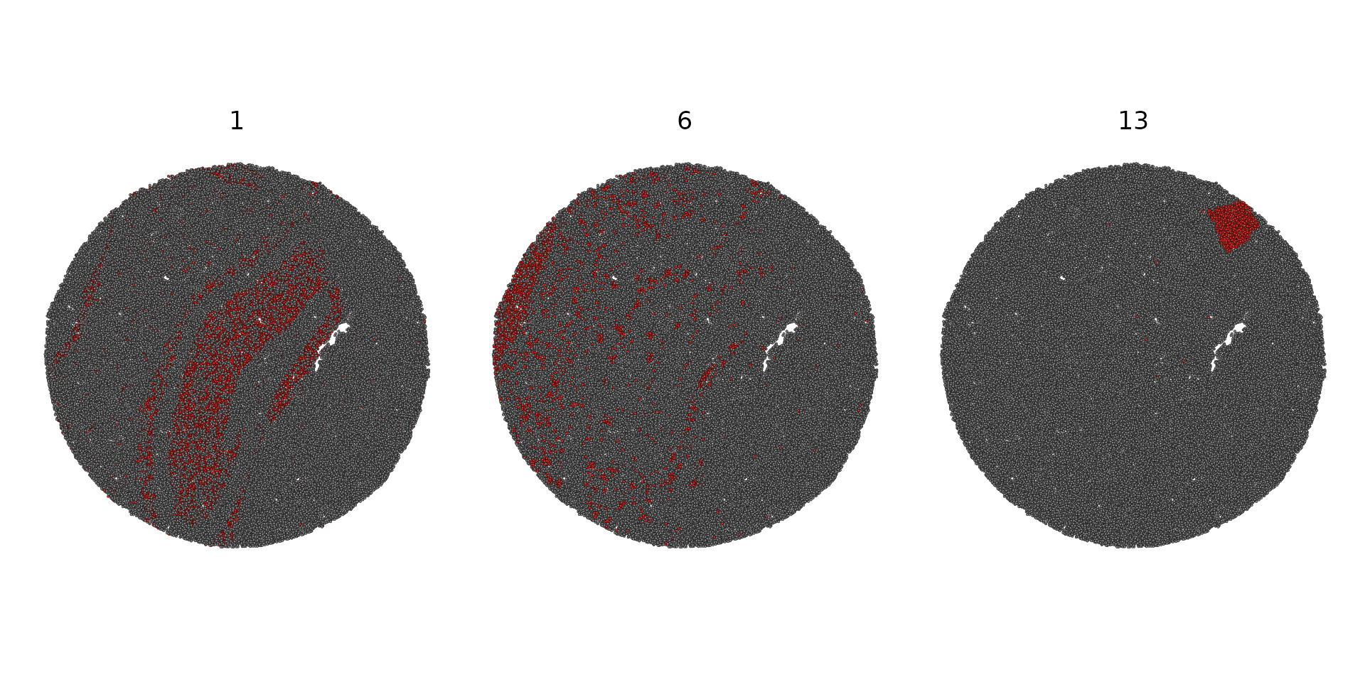
Integration with a scRNA-seq reference
To facilitate cell-type annotation of the Slide-seq dataset, we are leveraging an existing mouse single-cell RNA-seq hippocampus dataset, produced in Saunders*, Macosko*, et al. 2018. The data is available for download as a processed Seurat object here, with the raw count matrices available on the DropViz website.
ref <- readRDS("/brahms/shared/vignette-data/mouse_hippocampus_reference.rds")
ref <- UpdateSeuratObject(ref)
The original annotations from the paper are provided in the cell
metadata of the Seurat object. These annotations are provided at several
“resolutions”, from broad classes (ref$class) to
subclusters within celltypes (ref$subcluster). For the
purposes of this vignette, we work off of a modification of the celltype
annotations (ref$celltype) which we feel strikes a good
balance.
We’ll start by running the Seurat label transfer method to predict the major celltype for each bead.
anchors <- FindTransferAnchors(reference = ref,
                               query = slide.seq,
                               normalization.method = "SCT",
                               npcs = 50)

predictions.assay <- TransferData(anchorset = anchors,
                                  refdata = ref$celltype,
                                  prediction.assay = TRUE,
                                  weight.reduction = slide.seq[["pca"]],
                                  dims = 1:50)

slide.seq[["predictions"]] <- predictions.assay
We can then visualize the prediction scores for some of the major expected classes.
DefaultAssay(slide.seq) <- "predictions"

cell.types.of.interest <- c("CA3 Principal cells", "Dentate Principal cells", "Endothelial tip", "Entorhinal cortex", "Ependymal", "Oligodendrocyte")

SpatialFeaturePlot(slide.seq, features = cell.types.of.interest, alpha = c(0.1, 1))![]()
slide.seq$predicted.id <- GetTransferPredictions(slide.seq)

Idents(slide.seq) <- "predicted.id"

cell.types.highlight <- CellsByIdentities(object = slide.seq, idents = cell.types.of.interest[1:3])

SpatialDimPlot(slide.seq, cells.highlight = cell.types.highlight, facet.highlight = TRUE)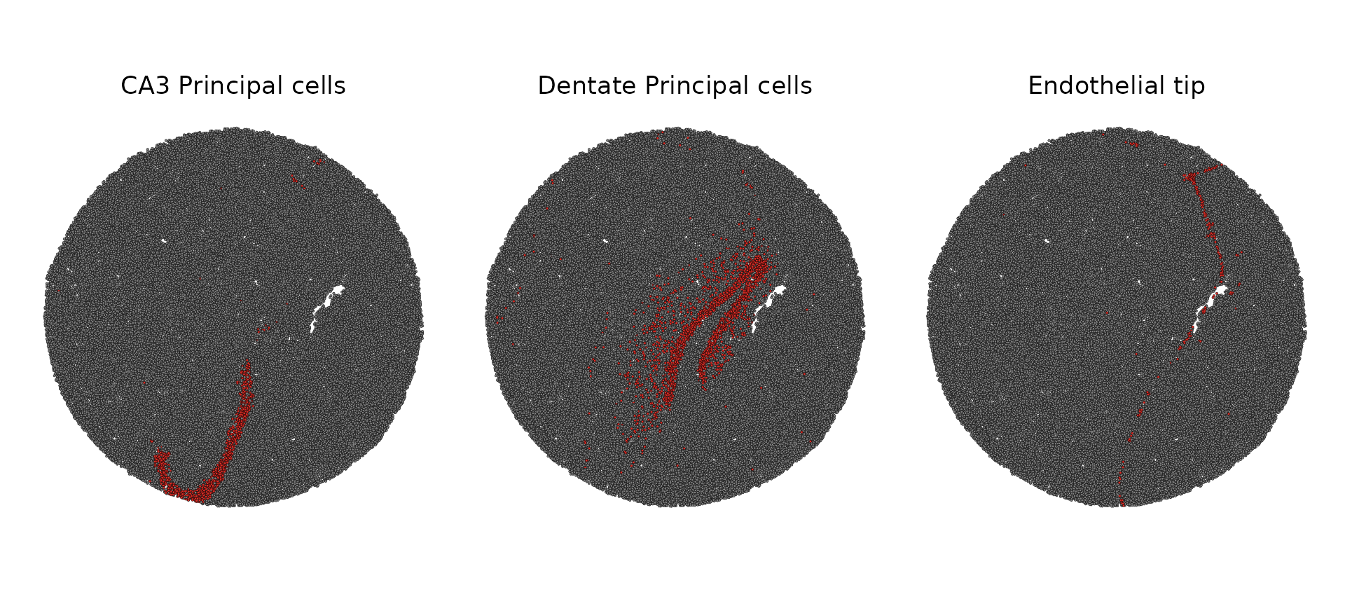
Identification of Spatially Variable Features
As mentioned above in the Visium vignette, we can identify spatially variable features in two general ways: differential expression testing between pre-annotated anatomical regions or statistics that measure the dependence of a feature on spatial location.
Here, we demonstrate the latter with an implementation of Moran’s I
available via FindSpatiallyVariableFeatures() by
setting method = "moransi". Moran’s I computes an overall
spatial autocorrelation and gives a statistic (similar to a correlation
coefficient) that measures the dependence of a feature on spatial
location. This allows us to rank features based on how spatially
variable their expression is.
In order to facilitate quick estimation of this statistic, we
implemented a basic binning strategy that will draw a rectangular grid
over a Slide-seq puck and average the feature and location within each
bin. The number of bins in the x and y direction are controlled by
the x.cuts and y.cuts parameters,
respectively. Additionally, while not required, installing the
optional Rfast2 package will significantly decrease the
runtime via a more efficient implementation.
DefaultAssay(slide.seq) <- "SCT"

slide.seq <- FindSpatiallyVariableFeatures(slide.seq,
                                           assay = "SCT",
                                           layer = "scale.data",
                                           features = VariableFeatures(slide.seq)[1:1000],
                                           selection.method = "moransi",
                                           x.cuts = 100, y.cuts = 100)
Now we visualize the expression of the top 6 features identified by Moran’s I.
spatially.variable.feats <- SpatiallyVariableFeatures(slide.seq, method = "moransi")

SpatialFeaturePlot(slide.seq,
                   features = head(spatially.variable.feats, 6),
                   ncol = 3,
                   alpha = c(0.1, 1),
                   max.cutoff = "q95")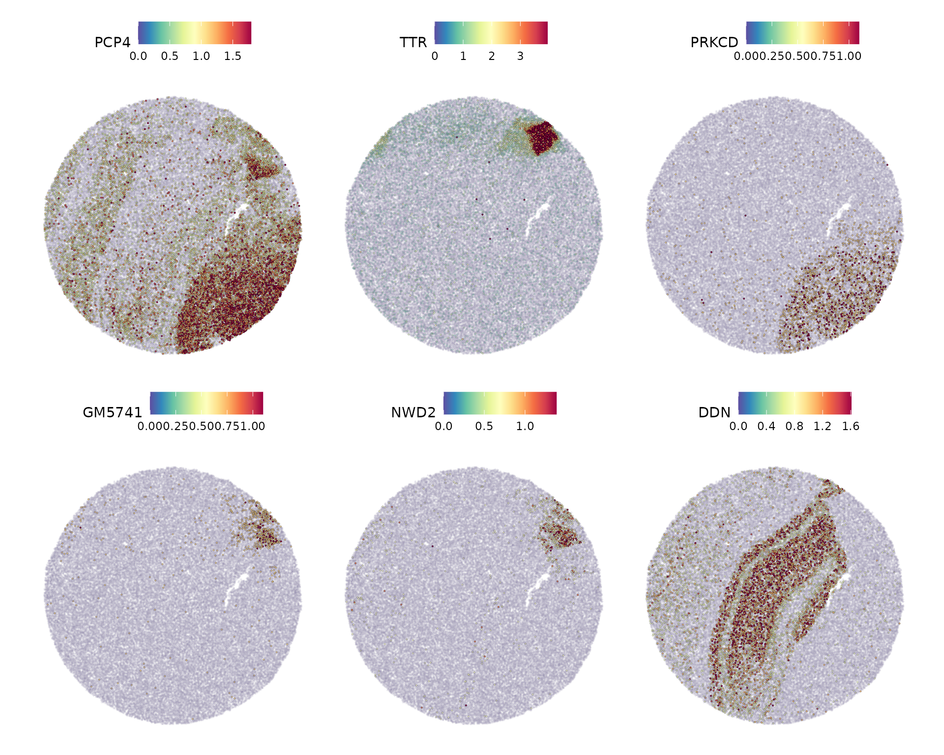
Spatial deconvolution using RCTD
While FindTransferAnchors can be used to integrate
spot-level data from spatial transcriptomic datasets, Seurat v5 also
includes support for the Robust Cell
Type Decomposition, a computational approach to deconvolve
spot-level data from spatial datasets, when provided with an scRNA-seq
reference. RCTD has been shown to accurately annotate spatial data from
a variety of technologies, including SLIDE-seq, Visium, and the 10x
Xenium in-situ spatial platform.
To run RCTD, we first install the spacexr package from
GitHub which implements RCTD.
devtools::install_github("dmcable/spacexr", build_vignettes = FALSE)Counts, cluster, and spot information is extracted from the Seurat
query and reference objects to construct Reference and
SpatialRNA objects used by RCTD for annotation.
library(spacexr)

# Set up reference
ref <- readRDS("/brahms/shared/vignette-data/mouse_hippocampus_reference.rds")
ref <- UpdateSeuratObject(ref)
Idents(ref) <- "celltype"

# Extract information to pass to the RCTD Reference function
counts <- ref[["RNA"]]$counts
cluster <- as.factor(ref$celltype)
names(cluster) <- colnames(ref)
nUMI <- ref$nCount_RNA
names(nUMI) <- colnames(ref)
reference <- Reference(counts, cluster, nUMI)

# Set up query with the RCTD function SpatialRNA
slide.seq <- SeuratData::LoadData("ssHippo")
counts <- slide.seq[["Spatial"]]$counts
coords <- GetTissueCoordinates(slide.seq)
colnames(coords) <- c("x", "y")
coords[is.na(colnames(coords))] <- NULL
query <- SpatialRNA(coords, counts, colSums(counts))
Using the reference and query object, we
annotate the dataset and add the cell type labels to the query Seurat
object. RCTD parallelizes well, so multiple cores can be specified for
faster performance.
RCTD <- create.RCTD(query, reference, max_cores = 8)
RCTD <- run.RCTD(RCTD, doublet_mode = 'doublet')
slide.seq <- AddMetaData(slide.seq, metadata = RCTD@results$results_df)
Next, plot the RCTD annotations. Because we ran RCTD in doublet mode,
the algorithm assigns a first_type and
second_type for each barcode or spot.
p1 <- SpatialDimPlot(slide.seq, group.by = "first_type")
p2 <- SpatialDimPlot(slide.seq, group.by = "second_type")

p1 | p2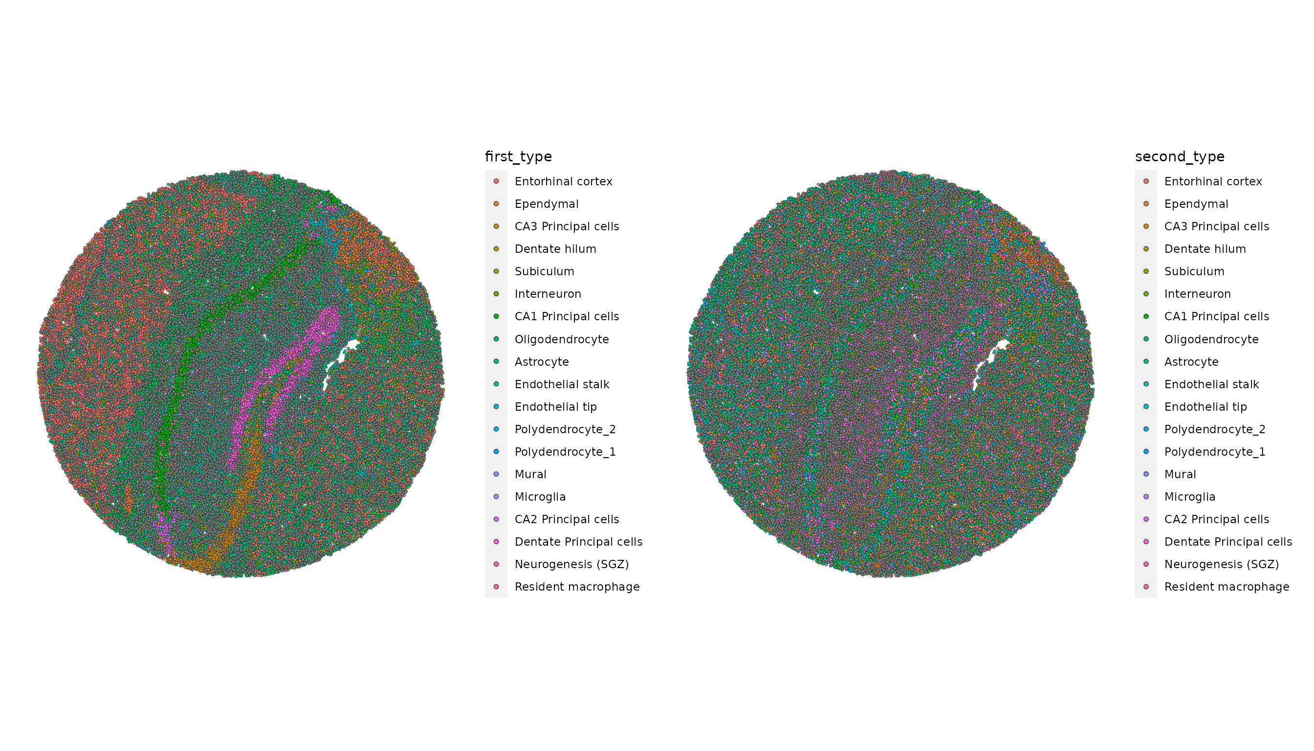
Session Info
## R version 4.5.2 (2025-10-31)
## Platform: x86_64-pc-linux-gnu
## Running under: Ubuntu 24.04.4 LTS
##
## Matrix products: default
## BLAS:   /usr/lib/x86_64-linux-gnu/openblas-pthread/libblas.so.3
## LAPACK: /usr/lib/x86_64-linux-gnu/openblas-pthread/libopenblasp-r0.3.26.so;  LAPACK version 3.12.0
##
## locale:
##  [1] LC_CTYPE=en_US.UTF-8       LC_NUMERIC=C
##  [3] LC_TIME=en_US.UTF-8        LC_COLLATE=en_US.UTF-8
##  [5] LC_MONETARY=en_US.UTF-8    LC_MESSAGES=en_US.UTF-8
##  [7] LC_PAPER=en_US.UTF-8       LC_NAME=C
##  [9] LC_ADDRESS=C               LC_TELEPHONE=C
## [11] LC_MEASUREMENT=en_US.UTF-8 LC_IDENTIFICATION=C
##
## time zone: Etc/UTC
## tzcode source: system (glibc)
##
## attached base packages:
## [1] stats     graphics  grDevices utils     datasets  methods   base
##
## other attached packages:
##  [1] spacexr_2.2.1             future_1.70.0
##  [3] vembedr_0.1.5             htmltools_0.5.9
##  [5] dplyr_1.2.0               patchwork_1.3.2
##  [7] ggplot2_4.0.3             stxBrain.SeuratData_0.1.2
##  [9] ssHippo.SeuratData_3.1.4  SeuratData_0.2.2.9002
## [11] Seurat_5.5.0              SeuratObject_5.4.0
## [13] sp_2.2-1
##
## loaded via a namespace (and not attached):
##   [1] RcppAnnoy_0.0.23            splines_4.5.2
##   [3] later_1.4.8                 tibble_3.3.1
##   [5] polyclip_1.10-7             fastDummies_1.7.6
##   [7] lifecycle_1.0.5             doParallel_1.0.17
##   [9] globals_0.19.1              Rnanoflann_0.0.3
##  [11] lattice_0.22-7              MASS_7.3-65
##  [13] magrittr_2.0.5              limma_3.66.0
##  [15] plotly_4.12.0               sass_0.4.10
##  [17] rmarkdown_2.30              jquerylib_0.1.4
##  [19] yaml_2.3.12                 httpuv_1.6.16
##  [21] otel_0.2.0                  glmGamPoi_1.22.0
##  [23] sctransform_0.4.3           spam_2.11-3
##  [25] spatstat.sparse_3.1-0       reticulate_1.46.0
##  [27] cowplot_1.2.0               pbapply_1.7-4
##  [29] RColorBrewer_1.1-3          abind_1.4-8
##  [31] quadprog_1.5-8              Rtsne_0.17
##  [33] GenomicRanges_1.62.1        purrr_1.2.1
##  [35] presto_1.0.0                BiocGenerics_0.56.0
##  [37] rappdirs_0.3.4              IRanges_2.44.0
##  [39] S4Vectors_0.48.1            ggrepel_0.9.8
##  [41] irlba_2.3.7                 listenv_0.10.1
##  [43] spatstat.utils_3.2-2        goftest_1.2-3
##  [45] RSpectra_0.16-2             spatstat.random_3.4-5
##  [47] fitdistrplus_1.2-6          parallelly_1.47.0
##  [49] pkgdown_2.2.0               DelayedMatrixStats_1.32.0
##  [51] codetools_0.2-20            DelayedArray_0.36.1
##  [53] tidyselect_1.2.1            farver_2.1.2
##  [55] matrixStats_1.5.0           stats4_4.5.2
##  [57] spatstat.explore_3.8-0      Seqinfo_1.0.0
##  [59] jsonlite_2.0.0              progressr_0.19.0
##  [61] iterators_1.0.14            ggridges_0.5.7
##  [63] survival_3.8-3              systemfonts_1.3.2
##  [65] foreach_1.5.2               tools_4.5.2
##  [67] ragg_1.5.1                  ica_1.0-3
##  [69] Rcpp_1.1.1-1.1              glue_1.8.0
##  [71] gridExtra_2.3               SparseArray_1.10.10
##  [73] xfun_0.56                   MatrixGenerics_1.22.0
##  [75] withr_3.0.2                 fastmap_1.2.0
##  [77] digest_0.6.39               R6_2.6.1
##  [79] mime_0.13                   textshaping_1.0.5
##  [81] scattermore_1.2             tensor_1.5.1
##  [83] dichromat_2.0-0.1           spatstat.data_3.1-9
##  [85] Rfast2_0.1.5.6              tidyr_1.3.2
##  [87] generics_0.1.4              data.table_1.18.2.1
##  [89] httr_1.4.8                  htmlwidgets_1.6.4
##  [91] S4Arrays_1.10.1             uwot_0.2.4
##  [93] pkgconfig_2.0.3             gtable_0.3.6
##  [95] lmtest_0.9-40               S7_0.2.1
##  [97] XVector_0.50.0              dotCall64_1.2
##  [99] zigg_0.0.2                  scales_1.4.0
## [101] Biobase_2.70.0              png_0.1-9
## [103] spatstat.univar_3.1-7       knitr_1.51
## [105] reshape2_1.4.5              nlme_3.1-168
## [107] cachem_1.1.0                zoo_1.8-15
## [109] stringr_1.6.0               KernSmooth_2.23-26
## [111] parallel_4.5.2              miniUI_0.1.2
## [113] vipor_0.4.7                 ggrastr_1.0.2
## [115] desc_1.4.3                  pillar_1.11.1
## [117] grid_4.5.2                  vctrs_0.7.1
## [119] RANN_2.6.2                  promises_1.5.0
## [121] beachmat_2.26.0             xtable_1.8-8
## [123] cluster_2.1.8.2             beeswarm_0.4.0
## [125] evaluate_1.0.5              cli_3.6.6
## [127] compiler_4.5.2              rlang_1.2.0
## [129] crayon_1.5.3                future.apply_1.20.2
## [131] labeling_0.4.3              plyr_1.8.9
## [133] fs_2.1.0                    ggbeeswarm_0.7.3
## [135] stringi_1.8.7               viridisLite_0.4.3
## [137] deldir_2.0-4                assertthat_0.2.1
## [139] lazyeval_0.2.3              spatstat.geom_3.7-3
## [141] Matrix_1.7-5                RcppHNSW_0.6.0
## [143] sparseMatrixStats_1.22.0    statmod_1.5.1
## [145] shiny_1.13.0                SummarizedExperiment_1.40.0
## [147] ROCR_1.0-12                 Rfast_2.1.5.2
## [149] igraph_2.3.0                RcppParallel_5.1.11-2
## [151] bslib_0.10.0
More specifically, this process calculates
gamma(r)values measuring the dependence between two spots a certain “r” distance apart. By default, we use an r-value of 5 in these analyses, and only compute these values for variable genes (where variation is calculated independently of spatial location) to save time.↩︎