Analysis and visualization of Visium HD data with cell segmentations in Seurat
Compiled: May 26, 2026
Source:vignettes/visiumhd_analysis_cell_segmentations.Rmd
visiumhd_analysis_cell_segmentations.RmdOverview
Traditional methods in spatial transcriptomics use bins typically ranging in size to approximate spatial locations of transcripts; however, binning approaches lose single-cell resolution. Released in June 2025, 10x Genomics’ Space Ranger cell segmentation workflow supports nucleus and cell segmentation for Visium HD and Visium HD 3’ H&E samples, allowing transcripts to be assigned at the cell level.
The segmentation approach involves capturing gene expression at subcellular resolution () and performing nuclei detection and expansion, which enables the delineation of individual cell boundaries. This allows much finer profiling of features, with gene counts reported on a per-cell basis rather than aggregated in or squares. For more information, see documentation from 10x.
With Seurat v5.4+, we introduce support for these new high-resolution datasets from Space Ranger, including the ability to:
- Load, process, and visualize spatial gene expression with segmentation overlays,
- Represent cell centroids and polygonal boundaries as distinct datatypes, and
- Perform clustering and spatial domain identification at multiple resolutions within the same object.
Together, these developments power segmentation-level spatial transcriptomics analysis in Seurat.
This vignette demonstrates how to use Seurat to analyze Visium HD cell segmentations. The typical analysis pipeline for these data is identical to those introduced in previous spatial vignettes; as such, here we aim to highlight the advantages of performing analyses at the cell level rather than at the spot or bin level, especially for complex and heterogeneous tissue architectures.
First, we load Seurat and the other packages necessary for this vignette. Core functionality in support of Visium HD cell segmentation data was initially introduced in Seurat v5.4.0 & SeuratObject v5.3.0.
Load data
In this vignette, we will use a Visium HD dataset of the human kidney (cortex) analyzed with Space Ranger 4.0.1. The data is available for download from the 10x data repository here.How do we set up the data directory?
First, create a directory to hold the data.
Then, go to the “Output and supplemental files” tab in the link to the repository above to access the core output files. The “batch download” option gives curl and wget commands to download the data via the terminal.
wget https://cf.10xgenomics.com/samples/spatial-exp/4.0.1/Visium_HD_Human_Kidney_FFPE/Visium_HD_Human_Kidney_FFPE_binned_outputs.tar.gz

wget https://cf.10xgenomics.com/samples/spatial-exp/4.0.1/Visium_HD_Human_Kidney_FFPE/Visium_HD_Human_Kidney_FFPE_segmented_outputs.tar.gz

wget https://cf.10xgenomics.com/samples/spatial-exp/4.0.1/Visium_HD_Human_Kidney_FFPE/Visium_HD_Human_Kidney_FFPE_spatial.tar.gz

wget https://cf.10xgenomics.com/samples/spatial-exp/4.0.1/Visium_HD_Human_Kidney_FFPE/Visium_HD_Human_Kidney_FFPE_barcode_mappings.parquet

wget https://cf.10xgenomics.com/samples/spatial-exp/4.0.1/Visium_HD_Human_Kidney_FFPE/Visium_HD_Human_Kidney_FFPE_feature_slice.h5

wget https://cf.10xgenomics.com/samples/spatial-exp/4.0.1/Visium_HD_Human_Kidney_FFPE/Visium_HD_Human_Kidney_FFPE_metrics_summary.csv

wget https://cf.10xgenomics.com/samples/spatial-exp/4.0.1/Visium_HD_Human_Kidney_FFPE/Visium_HD_Human_Kidney_FFPE_molecule_info.h5
Next, extract the binned outputs (expression matrices for , , and resolution bins), segmented outputs (segmentation-based expression data and segmentation polygons), and spatial data (H&E tissue images and spatial coordinate mappings).
After downloading the data, we load it into Seurat using the
Load10X_Spatial() function. As introduced in previous
vignettes, this function reads in the output of the Space
Ranger count pipeline. As of Space Ranger 4.0+, the
count pipeline also automatically runs the segment pipeline
for Visium HD and Visium HD 3’ data. We specify which data to load with
the bin.size argument. By including
"polygons", we load the segmentation-based expression data
where transcripts are assigned to individual cells based on the nuclei
detection and cell boundary expansion method. In this vignette, we also
load the
-binned
data for comparison. More about the Load10X_Spatial arguments used
here
The image.name argument was also introduced in Seurat v5.4. Currently,
users specify either “tissue_lowres_image.png” (default) or
“tissue_hires_image.png”. The high-resolution image is 10 times larger,
so it is useful for generating higher quality visualizations; however,
users should also consider object size & analysis needs when
deciding what to load. The documentation for
Load10X_Spatial provides more details on other arguments
that may be of interest to users who want to customize their workflows.
path_to_data <- "/brahms/shared/vignette-data/visium_hd_human_kidney"

kidney_obj <- Load10X_Spatial(data.dir = path_to_data,
                              bin.size = c(8, "polygons"),
                              image.name = "tissue_hires_image.png")
We can inspect the images and their associated assays to verify the data stored in the object:
Images(kidney_obj)## [1] "slice1.008um" "slice1.polygons"
kidney_obj[["slice1.008um"]]## Spatial coordinates for 666695 cells
## Default segmentation boundary: centroids
## Associated assay: Spatial.008um
## Key: slice1008um_
kidney_obj[["slice1.polygons"]]## Spatial coordinates for 148056 cells
## Default segmentation boundary: centroids
## 1 other segmentation boundaries present: segmentations
## Associated assay: Spatial.Polygons
## Key: slice1polygons_Bins vs. segmentations
One of the key advantages of the segmentation approach is the ability to analyze and visualize data at single-cell resolution. Before we plot the data on the whole tissue image, we can first define regions of interest in the tissue image for focused analysis later.
In order to do so, we begin by inspecting the whole tissue image and its coordinate ranges.
tissue_image <- SpatialDimPlot(kidney_obj,
                               images = "slice1.008um",
                               alpha = 0,
                               image.scale = "hires") +
                    ggtitle("Tissue image") + NoLegend()

# Define layer to customize axis text
theme_layer <- theme(axis.text.x = element_text(size = 10, angle = 45),
                                    axis.text.y = element_text(size = 10),
                                    axis.title.x = element_text(size = 10),
                                    axis.title.y = element_text(size = 10))

tissue_image_with_axes <- tissue_image +
                              scale_x_continuous(n.breaks = 20) +
                              scale_y_reverse(n.breaks = 20) +
                              theme_layer

tissue_image_with_axes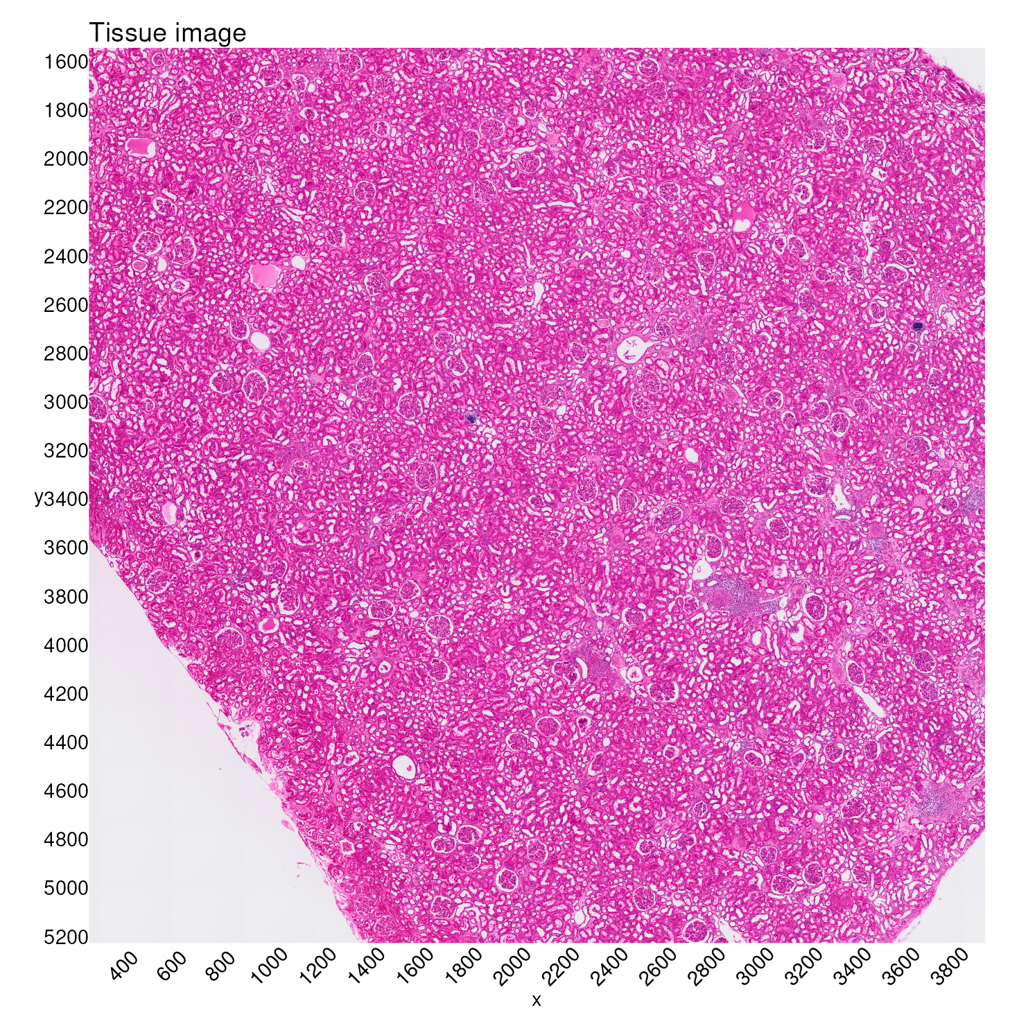
The approach we take here is to extract tissue coordinates and subset
our data to the same coordinate ranges for direct comparison.1 By using
Crop(),
we can define a new zoomed field of view (FOV), stored in the
images slot.
Here we define two different levels of zoom, based on coordinates from the tissue image above.
For the first level of zoom, we will take a section of pixels, and apply this to the segmented data.
zoom1_xlim <- c(2400, 3200)
zoom1_ylim <- c(3300, 3700)

kidney_obj[["zoom1.polygons"]] <- Crop(object = kidney_obj[["slice1.polygons"]],
                                              x = zoom1_xlim,
                                              y = zoom1_ylim,
                                              scale = "hires")
For the second level of zoom, we will take a smaller section of pixels, and apply this to both the binned and segmented data.
zoom2_xlim <- c(2750, 3150)
zoom2_ylim <- c(3350, 3650)

kidney_obj[["zoom2.polygons"]] <- Crop(object = kidney_obj[["slice1.polygons"]],
                                              x = zoom2_xlim,
                                              y = zoom2_ylim,
                                              scale = "hires")

kidney_obj[["zoom2.008um"]] <- Crop(object = kidney_obj[["slice1.008um"]],
                                           x = zoom2_xlim,
                                           y = zoom2_ylim,
                                           scale = "hires")
To see the regions captured in these zooms, we plot just the tissue:
tissue_image_zoom1 <- SpatialDimPlot(kidney_obj,
                                     images = "zoom1.polygons",
                                     alpha = 0,
                                     image.scale = "hires") +
                                  ggtitle("Zoom level 1") + NoLegend()

tissue_image_zoom2 <- SpatialDimPlot(kidney_obj,
                                     images = "zoom2.polygons",
                                     alpha = 0,
                                     image.scale = "hires") +
                                  ggtitle("Zoom level 2") + NoLegend()

tissue_image_zoom1 + tissue_image_zoom2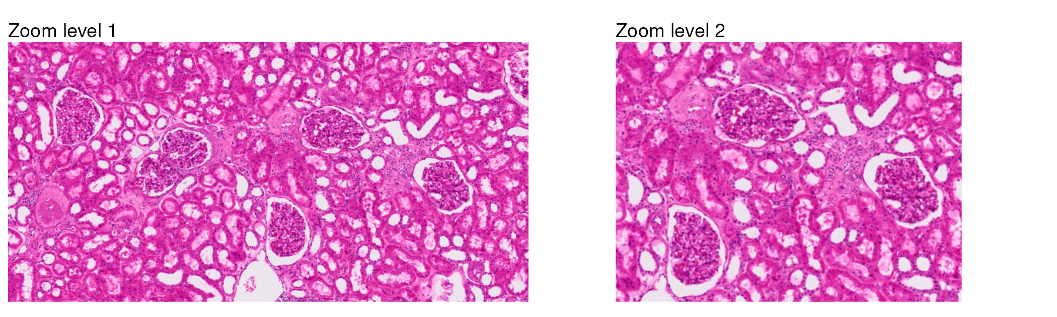
Now, we can take a closer look at how bins and cell segmentations capture spatial information by comparing how they appear when overlaid on the tissue image. Let’s use the second level of zoom for this comparison, since it is more focused on a smaller region of the tissue.
When generating a spatial plot of segmented data,
plot_segmentations = TRUE displays the full boundaries of
each segmentation polygon, rather than just the centroids. This allows
us to see the actual shape and size of each detected cell.
sdp_8um_zoom <- SpatialDimPlot(kidney_obj,
                               images = "zoom2.008um",
                               pt.size.factor = 18,
                               stroke = 0.1,
                               alpha = 0.6,
                               image.scale = "hires",
                               cols = "turquoise4") +
                    ggtitle("8µm bins") + NoLegend()

sdp_segm_zoom <- SpatialDimPlot(kidney_obj,
                                images = "zoom2.polygons",
                                plot_segmentations = TRUE,
                                stroke = 0.1,
                                alpha = 0.6,
                                image.scale = "hires",
                                cols = "turquoise4") +
                      ggtitle("Cell segmentations") + NoLegend()

sdp_8um_zoom + sdp_segm_zoom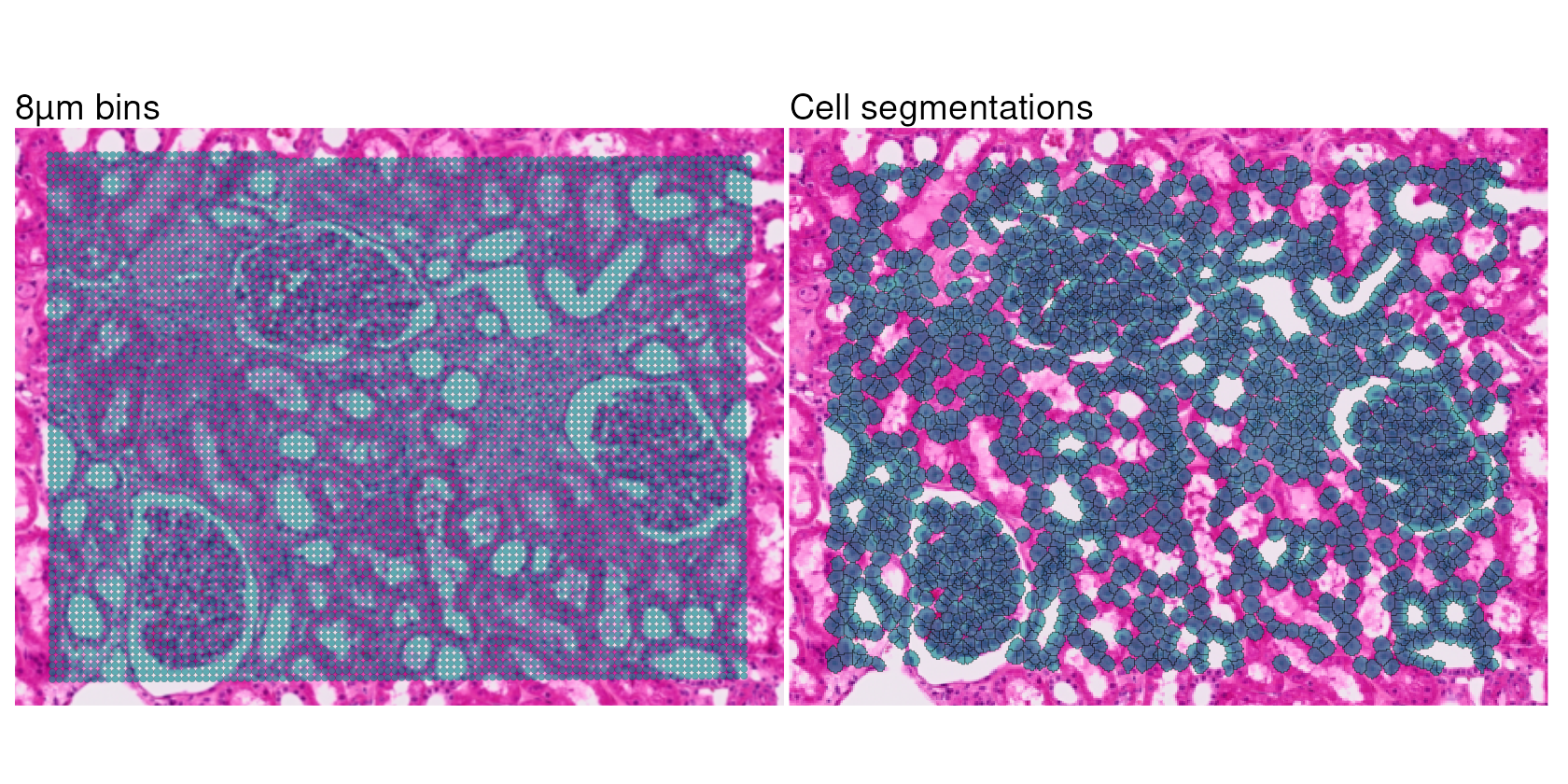
Cell type annotation with Pan-human Azimuth
We now annotate cell types in the segmentation-level data.
To perform cell type annotation, we use Pan-human Azimuth, a neural network-based classifier trained on a reference scRNA-seq dataset of 23 different types of human tissue. The classifier maps query cells to a hierarchical cell ontology and provides confidence scores for each annotation. The original implementation of this tool is in Python as panhumanpy.
In R, we can access Pan-human Azimuth through the AzimuthAPI package:
if (!requireNamespace("AzimuthAPI", quietly = TRUE)) {
  remotes::install_github("satijalab/AzimuthAPI")
}

library(AzimuthAPI)
Annotating cell segmentations
AzimuthAPI::CloudAzimuth() runs
Pan-human Azimuth on a Seurat object via a cloud-based API. The object
is returned with the results of cell type annotation as added cell-level
metadata, and the latent embeddings of the classifier as an added
dimensional reduction. For more details, see the Pan-human Azimuth R
API vignette.
We set the default assay, normalize the data with standard
log-normalization, and then run CloudAzimuth().
DefaultAssay(kidney_obj) <- "Spatial.Polygons"

kidney_obj <- NormalizeData(kidney_obj)
kidney_obj <- CloudAzimuth(kidney_obj,
                           assay = "Spatial.Polygons",
                           model_version = "v1")
First, we can inspect how the output of Pan-human Azimuth is stored
within the object metadata. Note that the object contains both
bins and cell segmentations; after running CloudAzimuth
above on the Spatial.Polygons assay, the Azimuth metadata
columns are populated for (only) cell segmentations.
| nCount_Spatial.Polygons | nFeature_Spatial.Polygons | full_hierarchical_labels | final_level_labels | final_level_confidence | full_consistent_hierarchy | azimuth_broad | azimuth_medium | azimuth_fine | azimuth_label | |
|---|---|---|---|---|---|---|---|---|---|---|
| cellid_000194058-1 | 671 | 541 | Epithelial cell|Epithelial cell of kidney|Renal intercalated cell|Type A intercalated cell | Type A intercalated cell | 0.5486034 | TRUE | Epithelial cell | False | Type A intercalated cell | Type A intercalated cell |
| cellid_000194060-1 | 511 | 444 | Perivascular cell|Pericyte | Pericyte | 0.9924289 | TRUE | Perivascular cell | Pericyte | Pericyte | Pericyte |
| cellid_000194061-1 | 814 | 659 | Epithelial cell|Epithelial cell of kidney|Renal epithelial cell - distal tubules | Renal epithelial cell - distal tubules | 0.8674310 | TRUE | Epithelial cell | Renal epithelial cell - distal tubules | Renal epithelial cell - distal tubules | Renal epithelial cell - distal tubules |
| cellid_000194068-1 | 335 | 189 | Fibroblast|Myofibroblast | Myofibroblast | 0.5834453 | TRUE | Fibroblast | Fibroblast | Myofibroblast | Myofibroblast |
| cellid_000194069-1 | 550 | 449 | Epithelial cell|Epithelial cell of kidney|Renal epithelial cell - distal tubules | Renal epithelial cell - distal tubules | 0.9853504 | TRUE | Epithelial cell | Renal epithelial cell - distal tubules | Renal epithelial cell - distal tubules | Renal epithelial cell - distal tubules |
| cellid_000194070-1 | 107 | 100 | Unassigned | Unassigned | 0.9084134 | TRUE | Immune cell | NA | NA | Unassigned |
We see that in addition to cell type annotations organized hierarchically, Pan-human Azimuth provides confidence scores for each annotation; lower confidence scores indicate uncertainty in hierarchy assignments. We can set a confidence threshold to retain only high-confidence annotations for downstream tasks.
In addition to using the confidence score as a QC metric for
annotation accuracy, we also encourage users to examine differentially
expressed genes for each annotated cell type with AzimuthAPI::make_azimuth_QC_heatmaps().
For example, we can look at a heatmap for cells annotated within the epithelial cell hierarchy:
kidney_azimuth_QC_heatmaps <- make_azimuth_QC_heatmaps(kidney_obj_hc)

kidney_azimuth_QC_heatmaps[["Epithelial cell_1"]]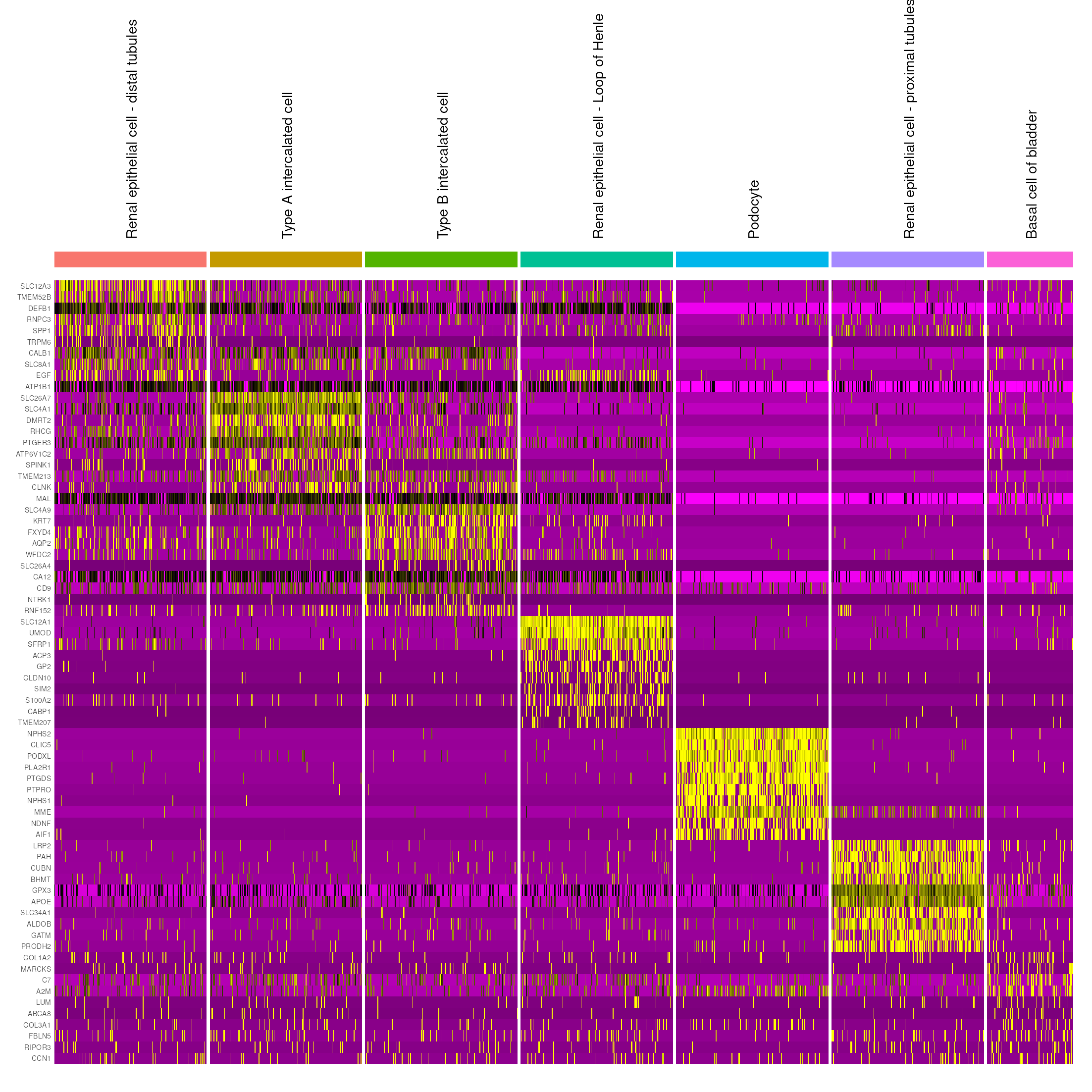
Additionally, the azimuth_embed dimensional reduction layer stores a 128-dimensional reduction of the Pan-human Azimuth embeddings. This is useful in downstream analyses. For example, we can visualize the cell type predictions returned by Pan-human Azimuth in embedding space:
kidney_obj_hc <- RunUMAP(kidney_obj_hc,
                         dims = 1:128,
                         reduction = "azimuth_embed",
                         reduction.name = "azimuth_umap")

p2 <- DimPlot(kidney_obj_hc,
              group.by = "final_level_labels",
              label.size = 2.5,
              label = TRUE,
              reduction = "azimuth_umap",
              repel = TRUE) + NoLegend()

p2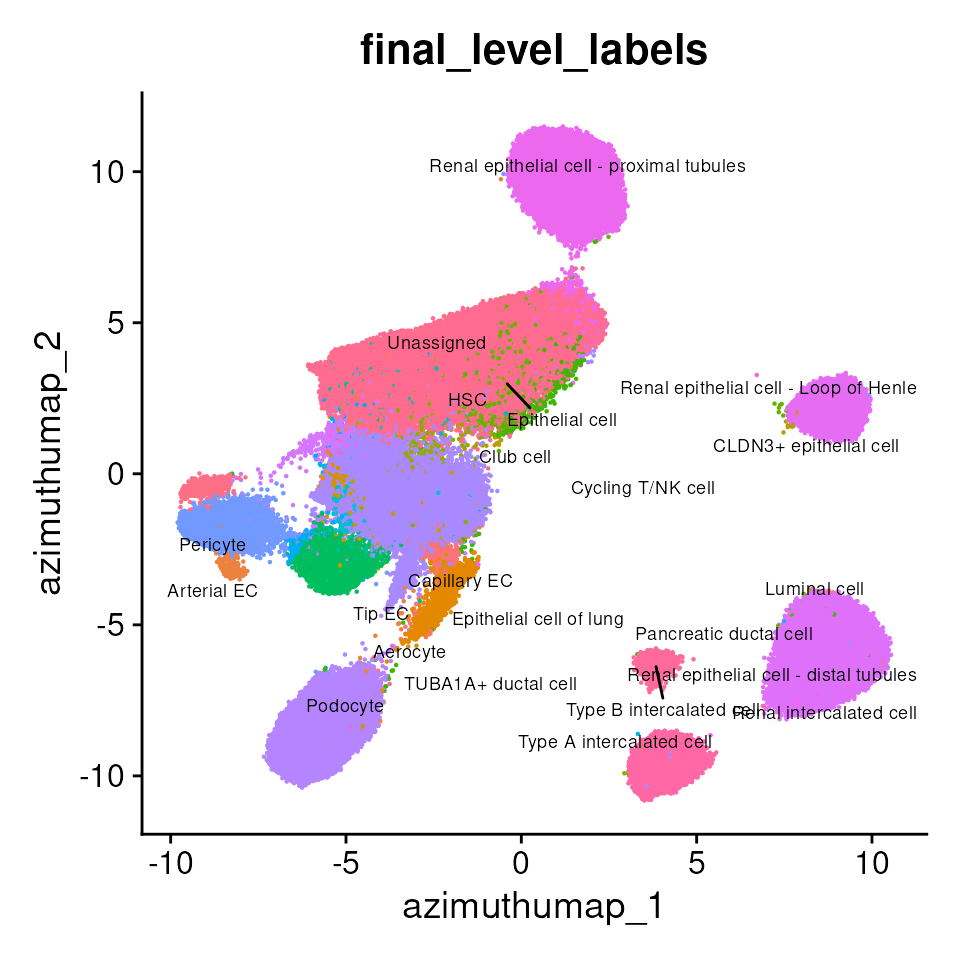
Cell type annotations in spatial context
Next, we can visualize where different cell types are located within the tissue. Mapping the cell type annotations onto the tissue image, we can observe the cell types present in various anatomically distinct regions2, such as glomeruli and renal tubules.
Podocytes are highly specialized cells found within the glomeruli of the kidney. We can focus our visualization on only cells annotated as podocytes:
kidney_segm_pod <- subset(kidney_obj_hc, final_level_labels == "Podocyte")

Idents(kidney_segm_pod) <- "final_level_labels"

pod_annotations_tissue <- SpatialDimPlot(kidney_segm_pod,
                                         images = "slice1.polygons",
                                         plot_segmentations = TRUE,
                                         image.scale = "hires",
                                         cols = "cyan") + NoLegend()

pod_annotations <- SpatialDimPlot(kidney_segm_pod,
                                  images = "slice1.polygons",
                                  image.alpha = 0,
                                  plot_segmentations = TRUE,
                                  image.scale = "hires",
                                  cols = "turquoise4") + NoLegend()

pod_annotations_tissue +
  pod_annotations +
  plot_annotation(title = 'Cells w/ annotation \'Podocyte\'')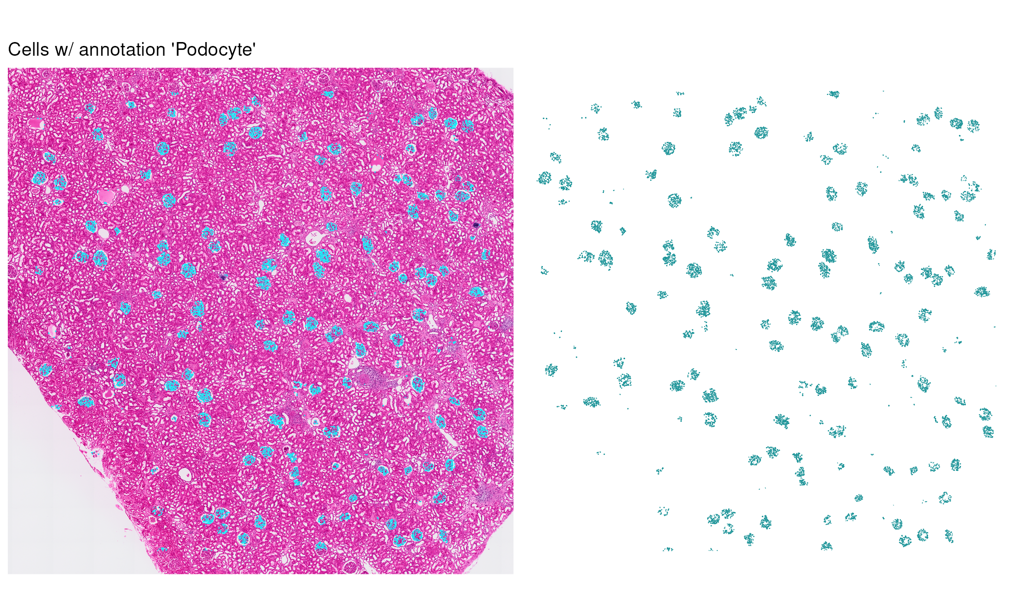
We can pick out some additional cell types of interest to examine the spatial organization of major kidney cell populations.
cell_types_of_interest <- c("Capillary EC",
                            "Pericyte",
                            "Podocyte",
                            "Renal epithelial cell - distal tubules",
                            "Renal epithelial cell - Loop of Henle",
                            "Type A intercalated cell",
                            "Type B intercalated cell")

kidney_segm_top <- subset(kidney_obj_hc,
                          final_level_labels %in% cell_types_of_interest)

Idents(kidney_segm_top) <- "final_level_labels"

cell_type_colors <- c("#06d31e", "#006326", "#000000", "#453494", "#ffaf01", "#00fffa", "#1da5f9")
names(cell_type_colors) <- cell_types_of_interest

full_image_annotated <- SpatialDimPlot(kidney_segm_top,
                                       images = "slice1.polygons",
                                       plot_segmentations = TRUE,
                                       alpha = 0.7,
                                       stroke = 0.04,
                                       image.scale = "hires",
                                       cols = cell_type_colors) +
                            labs(fill = "Cell type")

full_image_annotated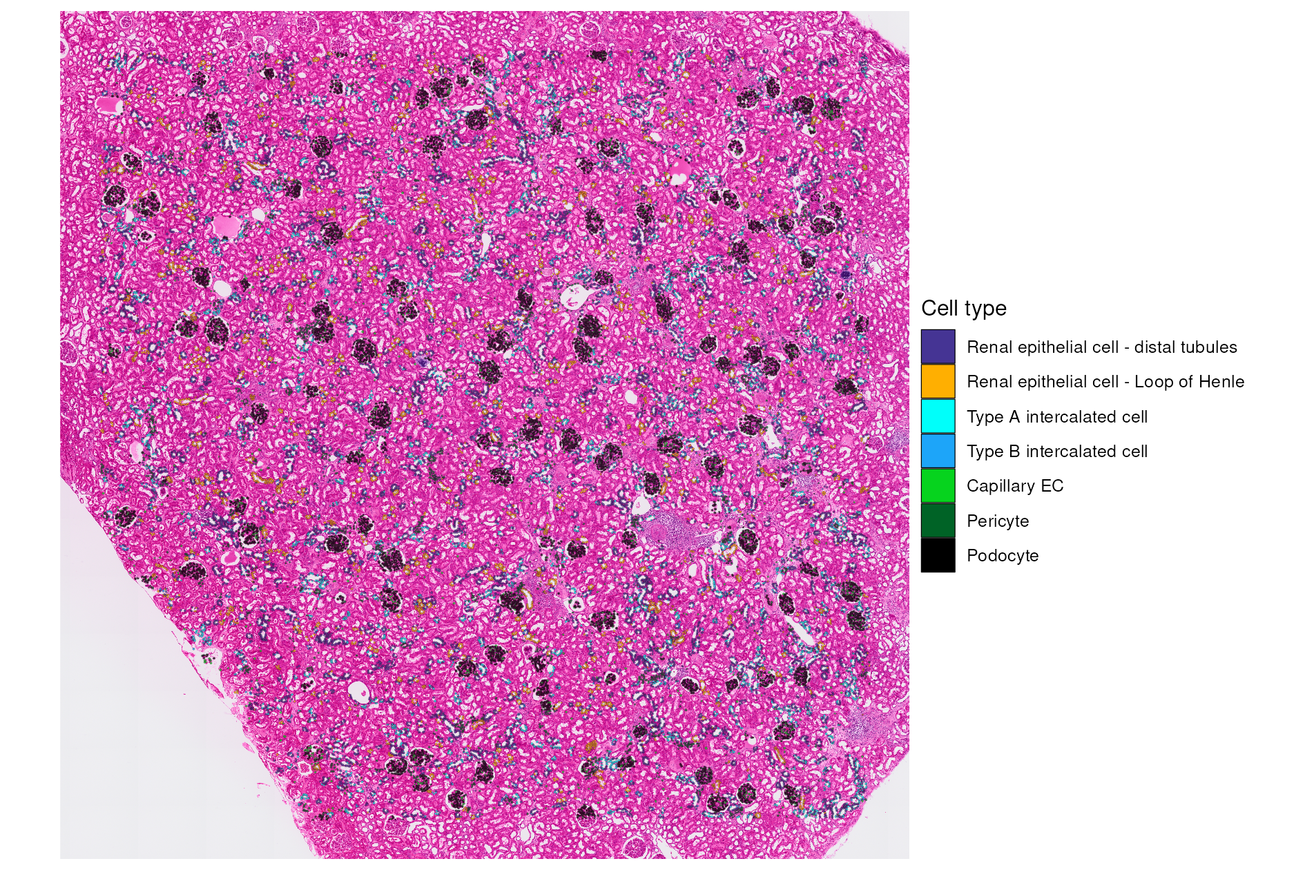
High-resolution zoom into tissue regions
Finally, zooming in again, we observe cell types annotated in and around some glomeruli.
# Define layers to customize the legend by putting it in three rows below the plot
legend_guide_layer <- list(theme(legend.position = "bottom",
                                 legend.text = element_text(size = 12),
                                 legend.title = element_blank()),
                           guides(fill = guide_legend(nrow = 3, byrow = TRUE)))

glom_zoom_annotated <- SpatialDimPlot(kidney_segm_top,
                                      images = "zoom1.polygons",
                                      group.by = "final_level_labels",
                                      plot_segmentations = TRUE,
                                      alpha = 0.7,
                                      stroke = 0.1,
                                      image.scale = "hires",
                                      cols = cell_type_colors) +
                            legend_guide_layer

glom_zoom_annotated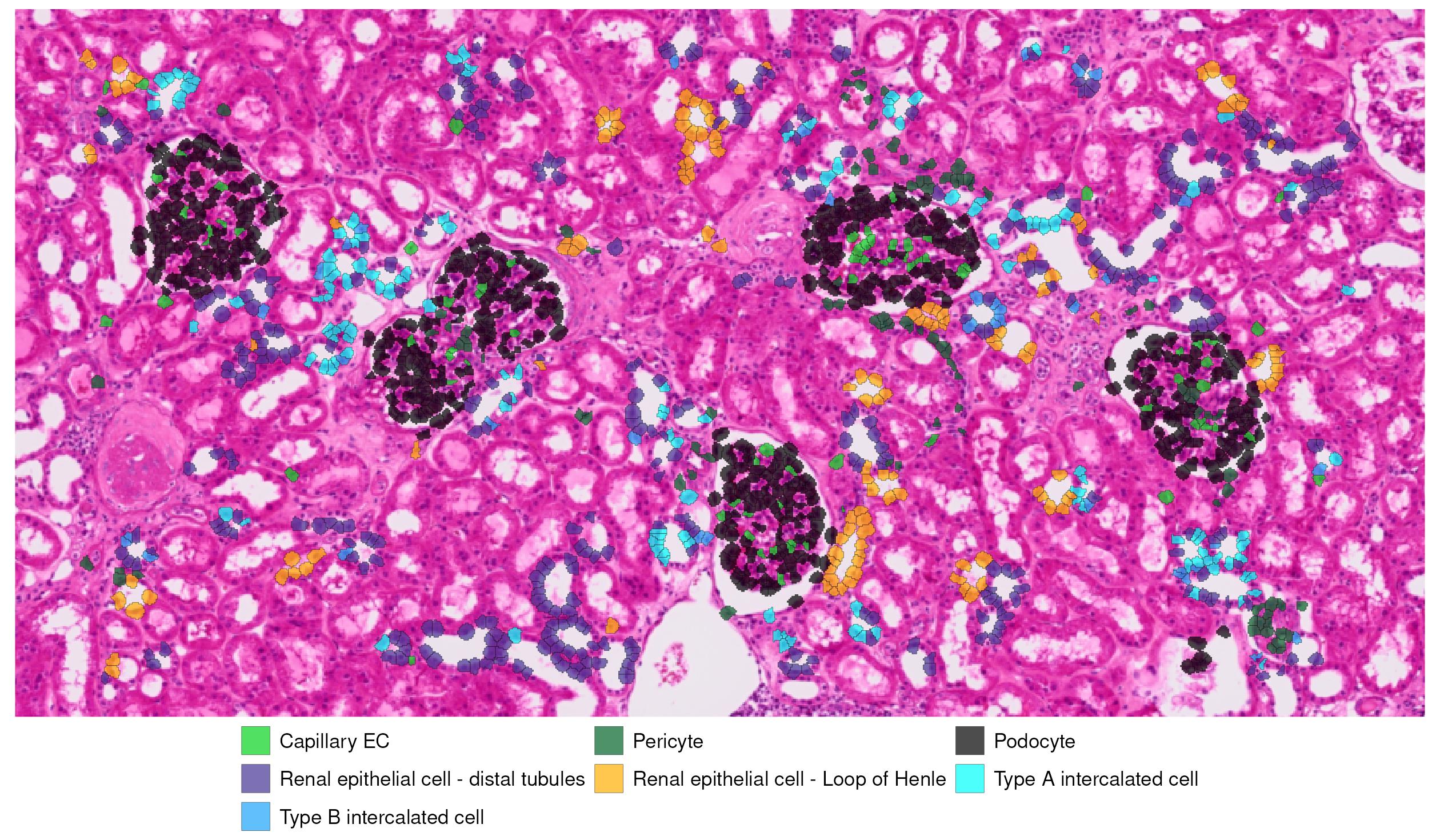
In this section of kidney cortex, which includes several glomeruli surrounded by renal tubules, the predicted cell type annotations align well with the underlying tissue structure. Podocytes are confined to the glomeruli, while endothelial and perivascular cells cluster within capillary-rich regions as expected. Distinct tubular epithelial populations are distributed along surrounding tubules, consistent with the normal spatial organization of nephron segments.
For more information on spatial analysis workflows, see the other spatial vignettes and documentation (Seurat, SeuratObject).
Acknowledgements
We would like to thank Stephen Williams and the Computational Biology team at 10x for their helpful feedback and contributions to the code for loading Visium segmentation data.
Session Info
## R version 4.5.2 (2025-10-31)
## Platform: x86_64-pc-linux-gnu
## Running under: Ubuntu 24.04.4 LTS
##
## Matrix products: default
## BLAS:   /usr/lib/x86_64-linux-gnu/openblas-pthread/libblas.so.3
## LAPACK: /usr/lib/x86_64-linux-gnu/openblas-pthread/libopenblasp-r0.3.26.so;  LAPACK version 3.12.0
##
## locale:
##  [1] LC_CTYPE=en_US.UTF-8       LC_NUMERIC=C
##  [3] LC_TIME=en_US.UTF-8        LC_COLLATE=en_US.UTF-8
##  [5] LC_MONETARY=en_US.UTF-8    LC_MESSAGES=en_US.UTF-8
##  [7] LC_PAPER=en_US.UTF-8       LC_NAME=C
##  [9] LC_ADDRESS=C               LC_TELEPHONE=C
## [11] LC_MEASUREMENT=en_US.UTF-8 LC_IDENTIFICATION=C
##
## time zone: Etc/UTC
## tzcode source: system (glibc)
##
## attached base packages:
## [1] stats     graphics  grDevices utils     datasets  methods   base
##
## other attached packages:
##  [1] knitr_1.51         AzimuthAPI_0.2.0   vembedr_0.1.5      htmltools_0.5.9
##  [5] dplyr_1.2.0        patchwork_1.3.2    ggplot2_4.0.3      Seurat_5.5.0
##  [9] SeuratObject_5.4.0 sp_2.2-1
##
## loaded via a namespace (and not attached):
##   [1] RColorBrewer_1.1-3     jsonlite_2.0.0         magrittr_2.0.5
##   [4] spatstat.utils_3.2-2   farver_2.1.2           rmarkdown_2.30
##   [7] fs_2.1.0               ragg_1.5.1             vctrs_0.7.1
##  [10] ROCR_1.0-12            spatstat.explore_3.8-0 RCurl_1.98-1.18
##  [13] curl_7.0.0             sass_0.4.10            sctransform_0.4.3
##  [16] parallelly_1.47.0      KernSmooth_2.23-26     bslib_0.10.0
##  [19] htmlwidgets_1.6.4      desc_1.4.3             ica_1.0-3
##  [22] plyr_1.8.9             plotly_4.12.0          zoo_1.8-15
##  [25] cachem_1.1.0           igraph_2.3.0           mime_0.13
##  [28] lifecycle_1.0.5        pkgconfig_2.0.3        Matrix_1.7-5
##  [31] R6_2.6.1               fastmap_1.2.0          fitdistrplus_1.2-6
##  [34] future_1.70.0          shiny_1.13.0           digest_0.6.39
##  [37] tensor_1.5.1           RSpectra_0.16-2        irlba_2.3.7
##  [40] textshaping_1.0.5      labeling_0.4.3         progressr_0.19.0
##  [43] spatstat.sparse_3.1-0  httr_1.4.8             polyclip_1.10-7
##  [46] abind_1.4-8            compiler_4.5.2         proxy_0.4-29
##  [49] bit64_4.6.0-1          withr_3.0.2            S7_0.2.1
##  [52] DBI_1.3.0              argparse_2.3.1         fastDummies_1.7.6
##  [55] MASS_7.3-65            classInt_0.4-11        units_1.0-1
##  [58] tools_4.5.2            lmtest_0.9-40          otel_0.2.0
##  [61] httpuv_1.6.16          future.apply_1.20.2    goftest_1.2-3
##  [64] glue_1.8.0             nlme_3.1-168           promises_1.5.0
##  [67] grid_4.5.2             sf_1.1-0               Rtsne_0.17
##  [70] cluster_2.1.8.2        reshape2_1.4.5         generics_0.1.4
##  [73] hdf5r_1.3.12           gtable_0.3.6           spatstat.data_3.1-9
##  [76] class_7.3-23           tidyr_1.3.2            data.table_1.18.2.1
##  [79] spatstat.geom_3.7-3    RcppAnnoy_0.0.23       ggrepel_0.9.8
##  [82] RANN_2.6.2             pillar_1.11.1          stringr_1.6.0
##  [85] limma_3.66.0           spam_2.11-3            RcppHNSW_0.6.0
##  [88] later_1.4.8            splines_4.5.2          lattice_0.22-7
##  [91] survival_3.8-3         bit_4.6.0              deldir_2.0-4
##  [94] tidyselect_1.2.1       miniUI_0.1.2           pbapply_1.7-4
##  [97] gridExtra_2.3          scattermore_1.2        xfun_0.56
## [100] statmod_1.5.1          matrixStats_1.5.0      stringi_1.8.7
## [103] lazyeval_0.2.3         yaml_2.3.12            evaluate_1.0.5
## [106] codetools_0.2-20       tibble_3.3.1           cli_3.6.6
## [109] uwot_0.2.4             arrow_23.0.1.2         xtable_1.8-8
## [112] reticulate_1.46.0      systemfonts_1.3.2      jquerylib_0.1.4
## [115] Rcpp_1.1.1-1.1         globals_0.19.1         spatstat.random_3.4-5
## [118] png_0.1-9              spatstat.univar_3.1-7  parallel_4.5.2
## [121] pkgdown_2.2.0          assertthat_0.2.1       presto_1.0.0
## [124] dotCall64_1.2          bitops_1.0-9           listenv_0.10.1
## [127] viridisLite_0.4.3      e1071_1.7-17           scales_1.4.0
## [130] ggridges_0.5.7         purrr_1.2.1            rlang_1.2.0
## [133] cowplot_1.2.0
For a purely visual comparison–without subsetting or creating a new FOV–with ggplot2 v4.0.0+ users can specify the desired
xlimandylimdirectly in acoord_fixed()layer on the plot of the whole tissue image.↩︎An introduction to the structure of the kidney cortex through an interactive view of normal tissue can be found via the Human Protein Atlas: https://www.proteinatlas.org/learn/dictionary/normal/kidney↩︎