Differential expression testing
Compiled: 2026-05-01
Source:vignettes/de_vignette.Rmd
de_vignette.RmdLoad in the data
This vignette highlights some example workflows for performing differential expression in Seurat. For demonstration purposes, we will be using the interferon-beta stimulated human PBMCs dataset (ifnb) that is available via the SeuratData package.
Perform default differential expression tests
The bulk of Seurat’s differential expression features can be accessed
through the FindMarkers() function. By default, Seurat
performs differential expression (DE) testing based on the
non-parametric Wilcoxon rank sum test. To test for DE genes between two
specific groups of cells, specify the ident.1 and
ident.2 parameters.
# Normalize the data
ifnb <- NormalizeData(ifnb)

# Find DE features between CD16 Mono and CD14 Mono
Idents(ifnb) <- "seurat_annotations"
monocyte.de.markers <- FindMarkers(ifnb, ident.1 = "CD16 Mono", ident.2 = "CD14 Mono")
# view results
head(monocyte.de.markers)
## p_val avg_log2FC pct.1 pct.2 p_val_adj
## VMO1 0.00000e+00 5.700274 0.778 0.084 0.000000e+00
## MS4A4A 0.00000e+00 3.349751 0.748 0.143 0.000000e+00
## FCGR3A 0.00000e+00 3.281942 0.982 0.418 0.000000e+00
## MS4A7 0.00000e+00 2.386436 0.978 0.558 0.000000e+00
## RPS19 0.00000e+00 1.325013 0.999 0.965 0.000000e+00
## CXCL16 6.82731e-317 2.014758 0.938 0.475 9.594419e-313The results data frame has the following columns :
- p_val : p-value (unadjusted)
- avg_log2FC : log fold-change of the average expression between the two groups. Positive values indicate that the feature is more highly expressed in the first group.
- pct.1 : The percentage of cells where the feature is detected in the first group
- pct.2 : The percentage of cells where the feature is detected in the second group
- p_val_adj : Adjusted p-value, based on Bonferroni correction using all features in the dataset.
If the ident.2 parameter is omitted or set to
NULL, FindMarkers() will test for
differentially expressed features between the group specified by
ident.1 and all other cells. Additionally, the parameter
only.pos can be set to TRUE to only search for
positive markers, i.e. features that are more highly expressed in the
ident.1 group.
# Find differentially expressed features between CD16 Monocytes and all other cells, only
# search for positive markers
monocyte.de.markers <- FindMarkers(ifnb, ident.1 = "CD16 Mono", ident.2 = NULL, only.pos = TRUE)
# view results
head(monocyte.de.markers)
## p_val avg_log2FC pct.1 pct.2 p_val_adj
## FCGR3A 0 4.532656 0.982 0.168 0
## MS4A7 0 3.806350 0.978 0.216 0
## CXCL16 0 3.274267 0.938 0.196 0
## VMO1 0 6.254651 0.778 0.044 0
## MS4A4A 0 4.747731 0.748 0.055 0
## LST1 0 2.927351 0.912 0.228 0Perform DE analysis within the same cell type across conditions
Since this dataset contains treatment information (control versus
stimulated with interferon-beta), we can also ask what genes change in
different conditions for cells of the same type. First, we create a
column in the meta.data slot to hold both the cell type and
treatment information and switch the current Idents to that
column. Then we use FindMarkers() to find the genes that
are different between control and stimulated CD14 monocytes.
ifnb$celltype.stim <- paste(ifnb$seurat_annotations, ifnb$stim, sep = "_")
Idents(ifnb) <- "celltype.stim"
mono.de <- FindMarkers(ifnb, ident.1 = "CD14 Mono_STIM", ident.2 = "CD14 Mono_CTRL", verbose = FALSE)
head(mono.de, n = 10)
## p_val avg_log2FC pct.1 pct.2 p_val_adj
## IFIT1 0 7.319139 0.985 0.033 0
## CXCL10 0 8.036564 0.984 0.035 0
## RSAD2 0 6.741673 0.988 0.045 0
## TNFSF10 0 6.991279 0.989 0.047 0
## IFIT3 0 6.883785 0.992 0.056 0
## IFIT2 0 7.179929 0.961 0.039 0
## CXCL11 0 8.624208 0.932 0.012 0
## CCL8 0 9.134191 0.918 0.017 0
## IDO1 0 5.455898 0.965 0.089 0
## MX1 0 5.059052 0.960 0.093 0However, the p-values obtained from this analysis should be interpreted with caution, because these tests treat each cell as an independent replicate and ignore inherent correlations between cells originating from the same sample. Such analyses have been shown to find a large number of false positive associations, as has been demonstrated by Squair et al., 2021, Zimmerman et al., 2021, Junttila et al., 2022, and others. Below, we show how pseudobulking can be used to account for such within-sample correlation.
Perform DE analysis after pseudobulking
To pseudobulk, we will use AggregateExpression() to sum together gene counts of all the cells from the same sample for each cell type. This results in one gene expression profile per sample and cell type. We can then perform DE analysis using DESeq2 on the sample level. This treats the samples, rather than the individual cells, as independent observations.
First, we need to retrieve the sample information for each cell. This is not loaded in the metadata, so we will load it from the Github repo of the source data for the original paper.
Add sample information to the dataset
# load the inferred sample IDs of each cell
ctrl <- read.table(url("https://raw.githubusercontent.com/yelabucsf/demuxlet_paper_code/master/fig3/ye1.ctrl.8.10.sm.best"), head = T, stringsAsFactors = F)
stim <- read.table(url("https://raw.githubusercontent.com/yelabucsf/demuxlet_paper_code/master/fig3/ye2.stim.8.10.sm.best"), head = T, stringsAsFactors = F)
info <- rbind(ctrl, stim)

# rename the cell IDs by substituting the '-' into '.'
info$BARCODE <- gsub(pattern = "\\-", replacement = "\\.", info$BARCODE)

# only keep the cells with high-confidence sample ID
info <- info[grep(pattern = "SNG", x = info$BEST), ]

# remove cells with duplicated IDs in both ctrl and stim groups
info <- info[!duplicated(info$BARCODE) & !duplicated(info$BARCODE, fromLast = T), ]

# now add the sample IDs to ifnb
rownames(info) <- info$BARCODE
info <- info[, c("BEST"), drop = F]
names(info) <- c("donor_id")
ifnb <- AddMetaData(ifnb, metadata = info)

# remove cells without donor IDs
ifnb$donor_id[is.na(ifnb$donor_id)] <- "unknown"
ifnb <- subset(ifnb, subset = donor_id != "unknown")
We can now perform pseudobulking (AggregateExpression())
based on the donor IDs.
# pseudobulk the counts based on donor-condition-celltype
pseudo_ifnb <- AggregateExpression(ifnb, assays = "RNA", return.seurat = T, group.by = c("stim", "donor_id", "seurat_annotations"))

# each 'cell' is a donor-condition-celltype pseudobulk profile
tail(Cells(pseudo_ifnb))
## [1] "STIM_SNG-1488_NK" "STIM_SNG-1488_DC"
## [3] "STIM_SNG-1488_B Activated" "STIM_SNG-1488_Mk"
## [5] "STIM_SNG-1488_pDC" "STIM_SNG-1488_Eryth"
pseudo_ifnb$celltype.stim <- paste(pseudo_ifnb$seurat_annotations, pseudo_ifnb$stim, sep = "_")Next, we perform DE testing on the pseudobulk level for CD14 monocytes, and compare it against the previous single-cell-level DE results.
Idents(pseudo_ifnb) <- "celltype.stim"

bulk.mono.de <- FindMarkers(object = pseudo_ifnb,
                         ident.1 = "CD14 Mono_STIM",
                         ident.2 = "CD14 Mono_CTRL",
                         test.use = "DESeq2")
head(bulk.mono.de, n = 15)
## p_val avg_log2FC pct.1 pct.2 p_val_adj
## IL1RN 3.701542e-275 5.588693 1 1 5.201777e-271
## IFITM2 1.955626e-250 4.108615 1 1 2.748242e-246
## SSB 2.699554e-203 2.893183 1 1 3.793684e-199
## NT5C3A 2.239898e-198 4.426872 1 1 3.147729e-194
## RTCB 5.700554e-162 2.738430 1 1 8.010989e-158
## RABGAP1L 4.743010e-161 4.494047 1 1 6.665352e-157
## DYNLT1 9.735640e-159 2.265511 1 1 1.368150e-154
## PLSCR1 3.191691e-146 2.501836 1 1 4.485284e-142
## ISG20 9.664488e-145 5.214558 1 1 1.358150e-140
## NAPA 2.858013e-144 1.782667 1 1 4.016365e-140
## DDX58 5.957026e-142 3.908225 1 1 8.371409e-138
## HERC5 6.333722e-133 4.360282 1 1 8.900780e-129
## OASL 3.892853e-130 3.691383 1 1 5.470627e-126
## EIF2AK2 6.636434e-128 3.386754 1 1 9.326180e-124
## TMEM50A 6.731955e-117 1.264359 1 1 9.460417e-113
# compare the DE P-values between the single-cell level and the pseudobulk level results
names(bulk.mono.de) <- paste0(names(bulk.mono.de), ".bulk")
bulk.mono.de$gene <- rownames(bulk.mono.de)

names(mono.de) <- paste0(names(mono.de), ".sc")
mono.de$gene <- rownames(mono.de)

merge_dat <- merge(mono.de, bulk.mono.de, by = "gene")
merge_dat <- merge_dat[order(merge_dat$p_val.bulk), ]

# Number of genes that are marginally significant in both; marginally significant only in bulk; and marginally significant only in single-cell
common <- merge_dat$gene[which(merge_dat$p_val.bulk < 0.05 &
                                merge_dat$p_val.sc < 0.05)]
only_sc <- merge_dat$gene[which(merge_dat$p_val.bulk > 0.05 &
                                  merge_dat$p_val.sc < 0.05)]
only_bulk <- merge_dat$gene[which(merge_dat$p_val.bulk < 0.05 &
                                    merge_dat$p_val.sc > 0.05)]
print(paste0('# Common: ',length(common)))
## [1] "# Common: 3519"## [1] "# Only in single-cell: 1649"## [1] "# Only in bulk: 204"We can see that while the p-values are correlated between the
single-cell and pseudobulk data, the single-cell p-values are often
smaller and suggest higher levels of significance. In particular, there
are 3,519 genes with evidence of differential expression (prior to
multiple hypothesis testing) in both analyses, 1,649 genes that only
appear to be differentially expressed in the single-cell analysis, and
just 204 genes that only appear to be differentially expressed in the
bulk analysis. We can investigate these discrepancies using
VlnPlot.
First, we can examine the top genes that are differentially expressed in both analyses.
# create a new column to annotate sample-condition-celltype in the single-cell dataset
ifnb$donor_id.stim <- paste0(ifnb$stim, "-", ifnb$donor_id)

# generate violin plot
Idents(ifnb) <- "celltype.stim"
print(merge_dat[merge_dat$gene%in%common[1:2],c('gene','p_val.sc','p_val.bulk')])
## gene p_val.sc p_val.bulk
## 2785 IL1RN 0 3.701542e-275
## 2739 IFITM2 0 1.955626e-250
VlnPlot(ifnb, features = common[1:2], idents = c("CD14 Mono_CTRL", "CD14 Mono_STIM"), group.by = "stim") 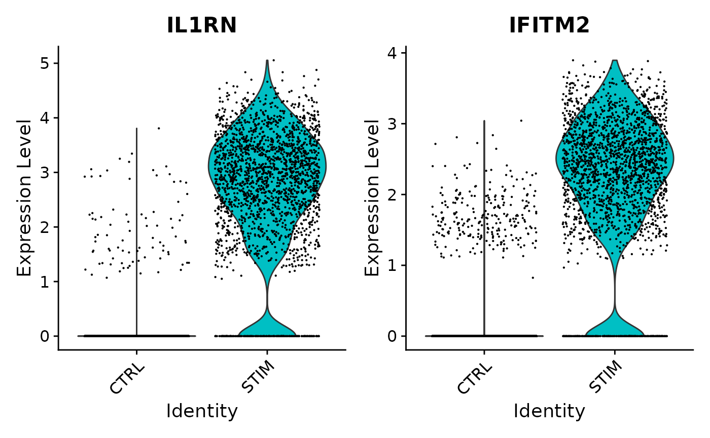
VlnPlot(ifnb, features = common[1:2], idents = c("CD14 Mono_CTRL", "CD14 Mono_STIM"), group.by = "donor_id.stim", ncol = 1) 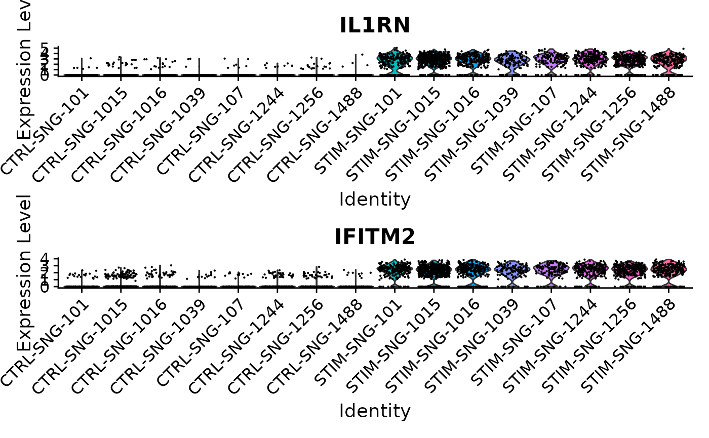
In both the pseudobulk and single-cell analyses, the p-values for these two genes are astronomically small. For both of these genes, when just comparing all stimulated CD14 monocytes to all control CD14 monocytes across samples, we see much higher expression in the stimulated cells. When breaking down these cells by sample, we continue to see consistently higher expression levels in the stimulated samples compared to the control samples; in other words, this finding is not driven by just one or two samples. Because of this consistency, we find this signal in both analyses.
By contrast, we can examine examples of genes that are only DE under the single-cell analysis.
##         gene     p_val.sc p_val.bulk
## 5710    SRGN 4.025076e-21  0.1823188
## 2603 HLA-DRA 4.989863e-09  0.1851302
VlnPlot(ifnb, features = c('SRGN','HLA-DRA'), idents = c("CD14 Mono_CTRL", "CD14 Mono_STIM"), group.by = "stim") 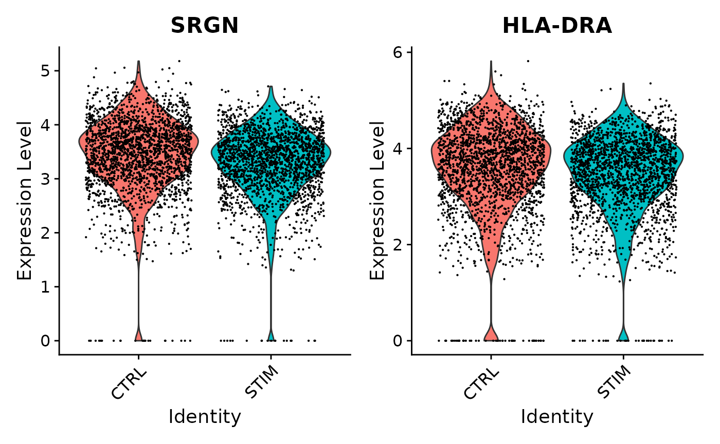
VlnPlot(ifnb, features = c('SRGN','HLA-DRA'), idents = c("CD14 Mono_CTRL", "CD14 Mono_STIM"), group.by = "donor_id.stim", ncol = 1) 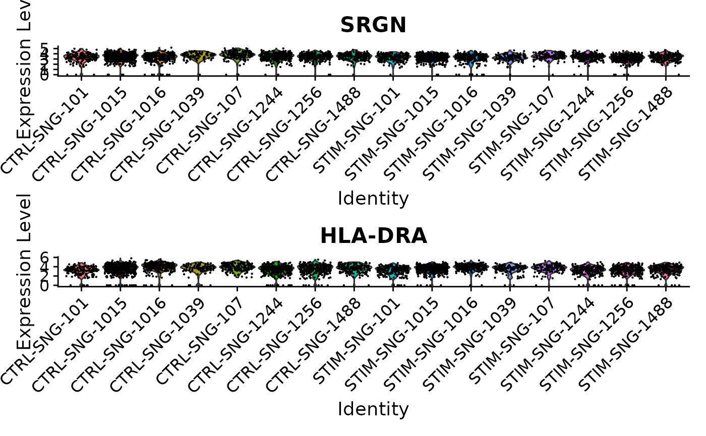
Here, SRGN and HLA-DRA both have very small p-values in the single-cell analysis (on the orders of and ), but much larger p-values around 0.18 in the pseudobulk analysis. While there appears to be a difference between control and stimulated cells when ignoring sample information, the signal is much weaker on the sample level, and we can see notable variability from sample to sample.
Perform DE analysis using alternative tests
Finally, we also support many other DE tests using other methods. For completeness, the following tests are currently supported:
- “wilcox” : Wilcoxon rank sum test (default, using ‘presto’ package)
- “wilcox_limma” : Wilcoxon rank sum test (using ‘limma’ package)
- “bimod” : Likelihood-ratio test for single cell feature expression, (McDavid et al., Bioinformatics, 2013)
- “roc” : Standard AUC classifier
- “t” : Student’s t-test
- “poisson” : Likelihood ratio test assuming an underlying negative binomial distribution. Use only for UMI-based datasets
- “negbinom” : Likelihood ratio test assuming an underlying negative binomial distribution. Use only for UMI-based datasets
- “LR” : Uses a logistic regression framework to determine differentially expressed genes. Constructs a logistic regression model predicting group membership based on each feature individually and compares this to a null model with a likelihood ratio test.
- “MAST” : GLM-framework that treats cellular detection rate as a covariate (Finak et al, Genome Biology, 2015) (Installation instructions)
- “DESeq2” : DE based on a model using the negative binomial
distribution (Love et al, Genome Biology, 2014) (Installation
instructions) For MAST and DESeq2, please ensure that these packages are
installed separately in order to use them as part of Seurat. Once
installed, the
test.useparameter can be used to specify which DE test to use.
# Test for DE features using the MAST package
Idents(ifnb) <- "seurat_annotations"
head(FindMarkers(ifnb, ident.1 = "CD14 Mono", ident.2 = "CD16 Mono", test.use = "MAST"))
Session Info
## R version 4.5.2 (2025-10-31)
## Platform: x86_64-pc-linux-gnu
## Running under: Ubuntu 24.04.4 LTS
##
## Matrix products: default
## BLAS:   /usr/lib/x86_64-linux-gnu/openblas-pthread/libblas.so.3
## LAPACK: /usr/lib/x86_64-linux-gnu/openblas-pthread/libopenblasp-r0.3.26.so;  LAPACK version 3.12.0
##
## locale:
##  [1] LC_CTYPE=en_US.UTF-8       LC_NUMERIC=C
##  [3] LC_TIME=en_US.UTF-8        LC_COLLATE=en_US.UTF-8
##  [5] LC_MONETARY=en_US.UTF-8    LC_MESSAGES=en_US.UTF-8
##  [7] LC_PAPER=en_US.UTF-8       LC_NAME=C
##  [9] LC_ADDRESS=C               LC_TELEPHONE=C
## [11] LC_MEASUREMENT=en_US.UTF-8 LC_IDENTIFICATION=C
##
## time zone: Etc/UTC
## tzcode source: system (glibc)
##
## attached base packages:
## [1] stats     graphics  grDevices utils     datasets  methods   base
##
## other attached packages:
## [1] ggplot2_4.0.3         ifnb.SeuratData_3.1.0 SeuratData_0.2.2.9002
## [4] Seurat_5.5.0          SeuratObject_5.4.0    sp_2.2-1
##
## loaded via a namespace (and not attached):
##   [1] RColorBrewer_1.1-3          jsonlite_2.0.0
##   [3] magrittr_2.0.5              ggbeeswarm_0.7.3
##   [5] spatstat.utils_3.2-2        farver_2.1.2
##   [7] rmarkdown_2.30              fs_2.1.0
##   [9] ragg_1.5.1                  vctrs_0.7.1
##  [11] ROCR_1.0-12                 spatstat.explore_3.8-0
##  [13] S4Arrays_1.10.1             htmltools_0.5.9
##  [15] SparseArray_1.10.10         sass_0.4.10
##  [17] sctransform_0.4.3           parallelly_1.47.0
##  [19] KernSmooth_2.23-26          bslib_0.10.0
##  [21] htmlwidgets_1.6.4           desc_1.4.3
##  [23] ica_1.0-3                   plyr_1.8.9
##  [25] plotly_4.12.0               zoo_1.8-15
##  [27] cachem_1.1.0                igraph_2.3.0
##  [29] mime_0.13                   lifecycle_1.0.5
##  [31] pkgconfig_2.0.3             Matrix_1.7-5
##  [33] R6_2.6.1                    fastmap_1.2.0
##  [35] MatrixGenerics_1.22.0       fitdistrplus_1.2-6
##  [37] future_1.70.0               shiny_1.13.0
##  [39] digest_0.6.39               S4Vectors_0.48.1
##  [41] patchwork_1.3.2             DESeq2_1.50.2
##  [43] tensor_1.5.1                RSpectra_0.16-2
##  [45] irlba_2.3.7                 GenomicRanges_1.62.1
##  [47] textshaping_1.0.5           labeling_0.4.3
##  [49] progressr_0.19.0            spatstat.sparse_3.1-0
##  [51] httr_1.4.8                  polyclip_1.10-7
##  [53] abind_1.4-8                 compiler_4.5.2
##  [55] withr_3.0.2                 S7_0.2.1
##  [57] BiocParallel_1.44.0         fastDummies_1.7.6
##  [59] MASS_7.3-65                 DelayedArray_0.36.1
##  [61] rappdirs_0.3.4              tools_4.5.2
##  [63] vipor_0.4.7                 lmtest_0.9-40
##  [65] otel_0.2.0                  beeswarm_0.4.0
##  [67] httpuv_1.6.16               future.apply_1.20.2
##  [69] goftest_1.2-3               glue_1.8.0
##  [71] nlme_3.1-168                promises_1.5.0
##  [73] grid_4.5.2                  Rtsne_0.17
##  [75] cluster_2.1.8.2             reshape2_1.4.5
##  [77] generics_0.1.4              gtable_0.3.6
##  [79] spatstat.data_3.1-9         tidyr_1.3.2
##  [81] data.table_1.18.2.1         XVector_0.50.0
##  [83] BiocGenerics_0.56.0         spatstat.geom_3.7-3
##  [85] RcppAnnoy_0.0.23            ggrepel_0.9.8
##  [87] RANN_2.6.2                  pillar_1.11.1
##  [89] stringr_1.6.0               spam_2.11-3
##  [91] RcppHNSW_0.6.0              limma_3.66.0
##  [93] later_1.4.8                 splines_4.5.2
##  [95] dplyr_1.2.0                 lattice_0.22-7
##  [97] survival_3.8-3              deldir_2.0-4
##  [99] tidyselect_1.2.1            locfit_1.5-9.12
## [101] miniUI_0.1.2                pbapply_1.7-4
## [103] knitr_1.51                  gridExtra_2.3
## [105] Seqinfo_1.0.0               IRanges_2.44.0
## [107] SummarizedExperiment_1.40.0 scattermore_1.2
## [109] stats4_4.5.2                xfun_0.56
## [111] Biobase_2.70.0              statmod_1.5.1
## [113] matrixStats_1.5.0           stringi_1.8.7
## [115] lazyeval_0.2.3              yaml_2.3.12
## [117] evaluate_1.0.5              codetools_0.2-20
## [119] tibble_3.3.1                cli_3.6.6
## [121] uwot_0.2.4                  xtable_1.8-8
## [123] reticulate_1.46.0           systemfonts_1.3.2
## [125] jquerylib_0.1.4             Rcpp_1.1.1-1.1
## [127] globals_0.19.1              spatstat.random_3.4-5
## [129] png_0.1-9                   ggrastr_1.0.2
## [131] spatstat.univar_3.1-7       parallel_4.5.2
## [133] pkgdown_2.2.0               presto_1.0.0
## [135] dotCall64_1.2               listenv_0.10.1
## [137] viridisLite_0.4.3           scales_1.4.0
## [139] ggridges_0.5.7              purrr_1.2.1
## [141] crayon_1.5.3                rlang_1.2.0
## [143] cowplot_1.2.0