Map COVID PBMC datasets to a healthy reference

library(Seurat)
library(BPCells)
library(dplyr)
library(patchwork)
library(ggplot2)
options(future.globals.maxSize = 10 * 1024^3)

Introduction: Reference mapping analysis in Seurat v5

In Seurat v5, we introduce a scalable approach for reference mapping datasets from separate studies or individuals. Reference mapping is a powerful approach to identify consistent labels across studies and perform cross-dataset analysis. We emphasize that while individual datasets are manageable in size, the aggregate of many datasets often amounts to millions of cell which do not fit in-memory. Furthermore, cross-dataset analysis is often challenged by disparate or unique cell type labels. Through reference mapping, we annotate all cells with a common reference for consistent cell type labels. Importantly, we never simultaneously load all of the cells in-memory to maintain low memory usage.

In this vignette, we reference map three publicly available datasets totaling 1,498,064 cells and 277 donors which are available through CZI cellxgene collections: Ahern, et al., Nature 2022, Jin, et al., Science 2021, and Yoshida, et al., Nature 2022. Each dataset consists of PBMCs from both healthy donors and donors diagnosed with COVID-19. Using the harmonized annotations, we demonstrate how to prepare a pseudobulk object to perform differential expression analysis across disease within cell types.

Prior to running this vignette, please install Seurat v5 and see the BPCells vignette to construct the on-disk object used in this vignette. Additionally, we map to our annotated CITE-seq reference containing 162,000 cells and 228 antibodies (Hao, Hao, et al., Cell 2021) which is available for download here.

Load the PBMC Reference Dataset and Query Datasets

We first load the reference (available here) and normalize the query Seurat object prepared in the BPCells interaction vignette. The query object consists of datasets from three different studies constructed using the CreateSeuratObject function, which accepts a list of BPCells matrices as input. Within the Seurat object, the three datasets reside in the RNA assay in three separate layers on-disk.

reference <- readRDS("/brahms/hartmana/vignette_data/pbmc_multimodal_2023.rds")
object <- readRDS("/brahms/mollag/seurat_v5/vignette_data/merged_covid_object.rds")
object <- NormalizeData(object, verbose = FALSE)

Mapping

Using the same code from the v4 reference mapping vignette, we find anchors between the reference and query in the precomputed supervised PCA. We recommend the use of supervised PCA for CITE-seq reference datasets, and demonstrate how to compute this transformation in v4 reference mapping vignette. In Seurat v5, we only need to call FindTransferAnchors and MapQuery once to map all three datasets as they are all contained within the query object. Furthermore, utilizing the on-disk capabilities of BPCells, we map 1.5 million cells without ever loading them all into memory.

anchor <- FindTransferAnchors(
  reference = reference,
  query = object,
  reference.reduction = 'spca',
  normalization.method = 'SCT',
  dims = 1:50)
object <- MapQuery(
  anchorset = anchor,
  query = object,
  reference = reference,
  refdata = list(
    celltype.l1 = "celltype.l1",
    celltype.l2 = "celltype.l2"
    ),
  reduction.model = 'wnn.umap'
)

Explore the mapping results

Next, we visualize all cells from the three studies which have been projected into a UMAP-space defined by the reference. Each cell is annotated at two levels of granularity (predicted.celltype.l1 and predicted.celltype.l2). We can compare the differing ontologies used in the original annotations (cell_type) to the now harmonized annotations (predicted.celltype.l2, for example) that were predicted from reference-mapping. Previously, the lack of standardization prevented us from directly performing integrative analysis across studies, but now we can easily compare.

DimPlot(object, reduction = 'ref.umap', group.by = 'cell_type',alpha = 0.1, label = TRUE, split.by = 'publication', ncol = 3,  label.size = 3) + NoLegend()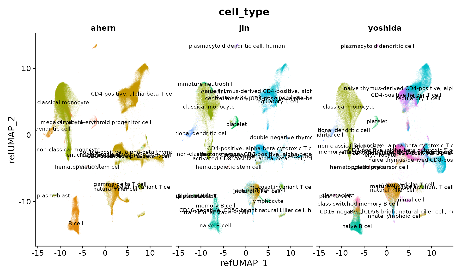

DimPlot(object, reduction = 'ref.umap', group.by = 'predicted.celltype.l2',alpha = 0.1, label = TRUE, split.by = 'publication', ncol = 3,  label.size = 3) + NoLegend()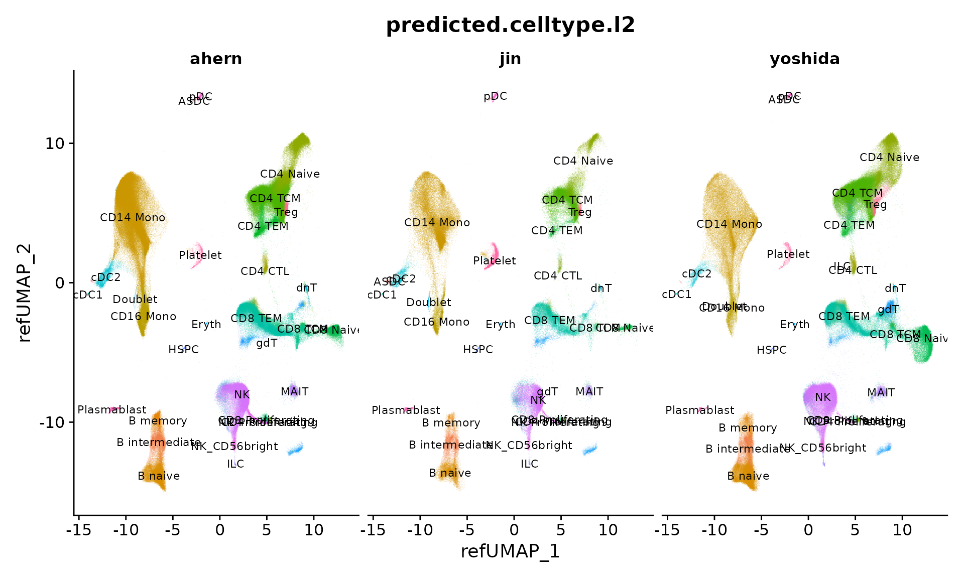

Differential composition analysis

We utilize our harmonized annotations to identify differences in the proportion of different cell types between healthy individuals and COVID-19 patients. For example, we noticed a reduction in MAIT cells as well as an increase in plasmablasts among COVID-19 patients.

df_comp <- as.data.frame.matrix(table(object$donor_id, object$predicted.celltype.l2))
select.donors <- rownames(df_comp)[rowSums(df_comp)> 50]
df_comp <- df_comp[select.donors, ]
df_comp_relative <- sweep(x = df_comp, MARGIN = 1, STATS = rowSums(df_comp), FUN = '/')

df_disease <-  as.data.frame.matrix(table(object$donor_id, object$disease))[select.donors, ]

df_comp_relative$disease <- 'other'
df_comp_relative$disease[df_disease$normal!=0] <- 'normal'
df_comp_relative$disease[df_disease$`COVID-19`!=0] <- 'COVID-19'
df_comp_relative$disease <- factor(df_comp_relative$disease, levels = c('normal','COVID-19','other'))
df_comp_relative <- df_comp_relative[df_comp_relative$disease %in% c('normal','COVID-19'),]

p1 <-  ggplot(data = df_comp_relative, mapping = aes(x = disease, y = MAIT, fill = disease)) +  
  geom_boxplot(outlier.shape  = NA) +
  scale_fill_manual(values = c("#377eb8", "#e41a1c")) +
  xlab("") + ylab('relative abundance') +
  ggtitle('MAIT') +
  geom_jitter(color="black", size=0.4, alpha=0.9 ) +
  theme_bw() +
  theme( axis.title = element_text(size = 12),
         axis.text = element_text(size = 12),
         plot.title = element_text(size = 15, hjust = 0.5, face = "bold")
  )

p2 <-  ggplot(data = df_comp_relative, mapping = aes(x = disease, y = Plasmablast, fill = disease)) +  
  geom_boxplot(outlier.shape  = NA) +
  scale_fill_manual(values = c("#377eb8", "#e41a1c")) +
  xlab("") + ylab('relative abundance') +
    ggtitle('Plasmablast') +
  geom_jitter(color="black", size=0.4, alpha=0.9 ) +
  theme_bw() +
  theme( axis.title = element_text(size = 12),
         axis.text = element_text(size = 12),
         plot.title = element_text(size = 15, hjust = 0.5, face = "bold")
  )

p1 + p2 + plot_layout(ncol = 2)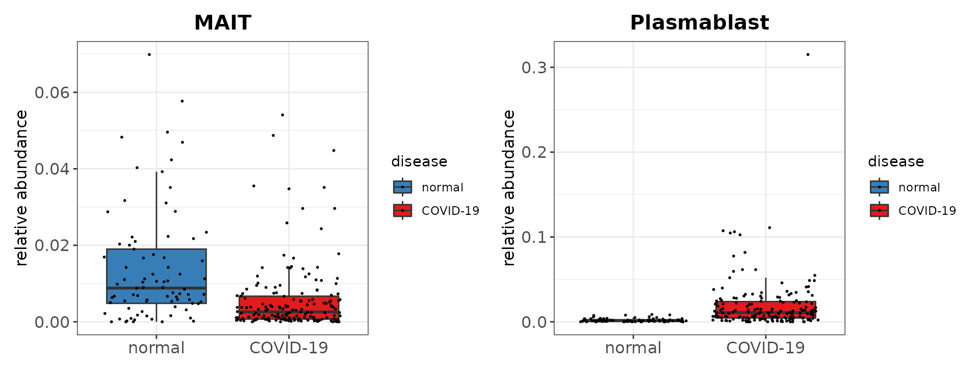

Differential expression analysis

In addition to composition analysis, we use an aggregation-based (pseudobulk) workflow to explore differential genes between healthy individuals and COVID-19 donors. We aggregate all cells within the same cell type and donor using the AggregateExpression function. This returns a Seurat object where each ‘cell’ represents the pseudobulk profile of one cell type in one individual.

bulk <- AggregateExpression(object,
  return.seurat = TRUE,
  assays  = 'RNA',
  group.by = c("predicted.celltype.l2", "donor_id", "disease")
)

bulk <- subset(bulk, subset = disease %in% c('normal', 'COVID-19') )
bulk <- subset(bulk, subset = predicted.celltype.l2 !=  'Doublet')
bulk$disease <- factor(bulk$disease, levels = c('normal', 'COVID-19'))

Once a pseudobulk object is created, we can perform cell type-specific differential expression analysis between healthy individuals and COVID-19 donors. Here, we only visualize certain interferon-stimulated genes which are often upregulated during viral infection.

p1 <- VlnPlot(
  object = bulk, features = 'IFI6', group.by = 'predicted.celltype.l2',
  split.by = 'disease', cols = c("#377eb8", "#e41a1c"))
p2 <- VlnPlot(
  object = bulk, features = c('ISG15'), group.by = 'predicted.celltype.l2',
  split.by = 'disease', cols = c("#377eb8", "#e41a1c"))
p3 <- VlnPlot(
  object = bulk, features = c('IFIT5'), group.by = 'predicted.celltype.l2',
  split.by = 'disease', cols = c("#377eb8", "#e41a1c"))
p1 + p2 + p3 + plot_layout(ncol = 1)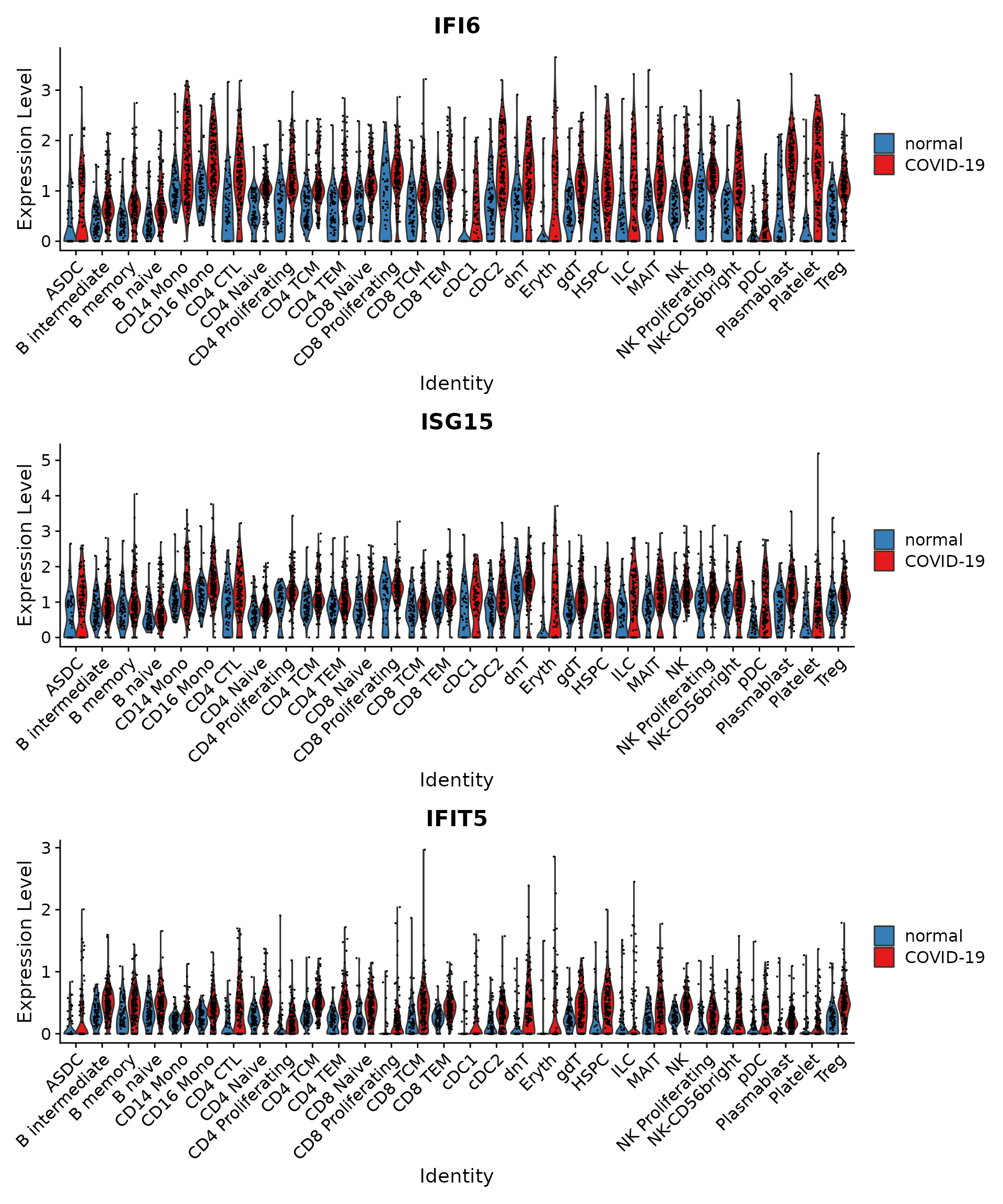

Session Info

sessionInfo()