Data visualization methods in Seurat
Compiled: April 28, 2026
Source:vignettes/visualization_vignette.Rmd
visualization_vignette.RmdHere, we demonstrate visualization techniques in Seurat using our previously computed Seurat object from the 2,700 PBMC guided clustering tutorial. You can access the dataset and load it into a Seurat object using SeuratData.
SeuratData::InstallData("pbmc3k")
library(Seurat)
library(SeuratData)
library(ggplot2)
library(patchwork)
pbmc3k.final <- LoadData("pbmc3k", type = "pbmc3k.final")
pbmc3k.final$groups <- sample(c("group1", "group2"), size = ncol(pbmc3k.final), replace = TRUE)
features <- c("LYZ", "CCL5", "IL32", "PTPRCAP", "FCGR3A", "PF4")
pbmc3k.final
## An object of class Seurat
## 13714 features across 2638 samples within 1 assay
## Active assay: RNA (13714 features, 2000 variable features)
## 3 layers present: data, counts, scale.data
## 2 dimensional reductions calculated: pca, umapFive visualizations of marker feature expression
# Ridge plots - from ggridges. Visualize single cell expression distributions in each cluster
RidgePlot(pbmc3k.final, features = features, ncol = 2)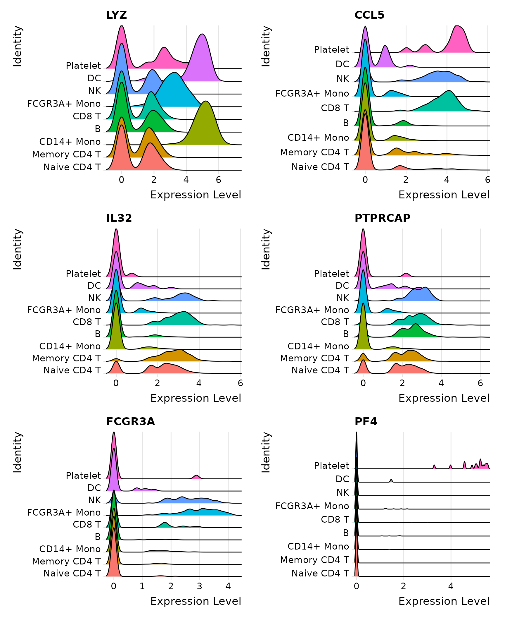
# Violin plot - Visualize single cell expression distributions in each cluster
VlnPlot(pbmc3k.final, features = features)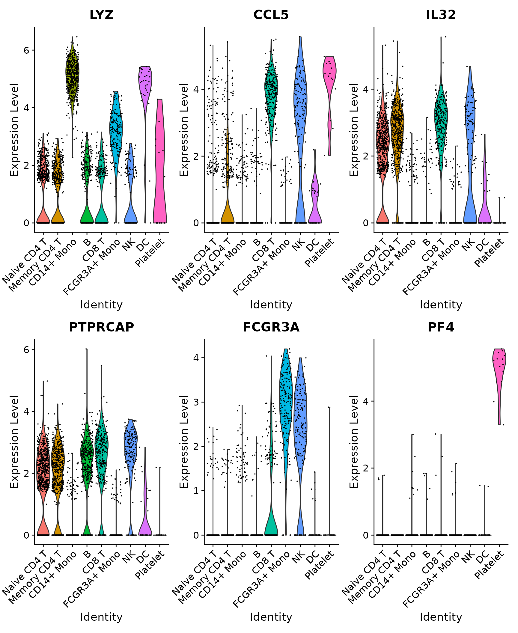
# Feature plot - visualize feature expression in low-dimensional space
FeaturePlot(pbmc3k.final, features = features)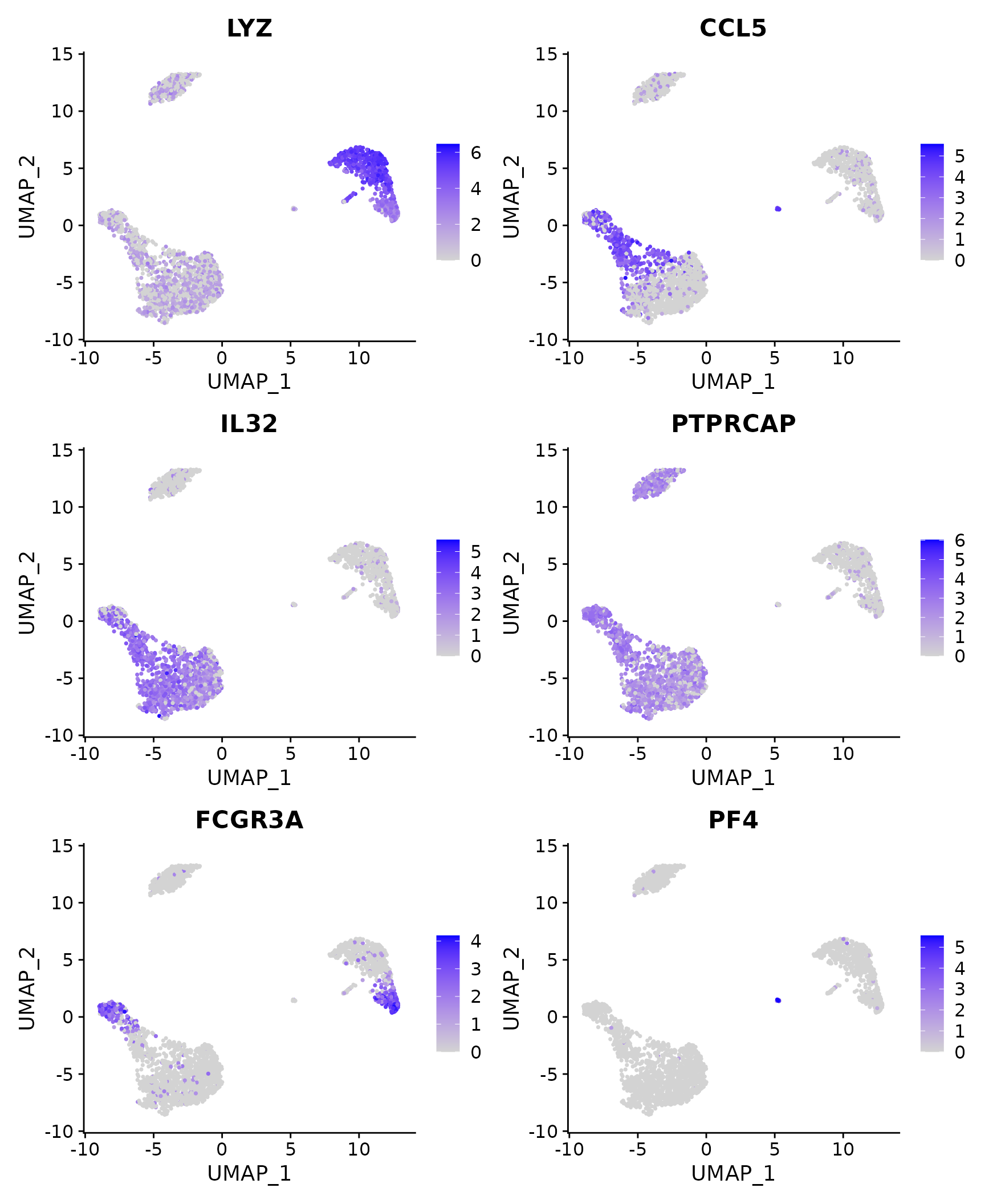
# Dot plots - the size of the dot corresponds to the percentage of cells expressing the
# feature in each cluster. The color represents the average expression level
DotPlot(pbmc3k.final, features = features) + RotatedAxis()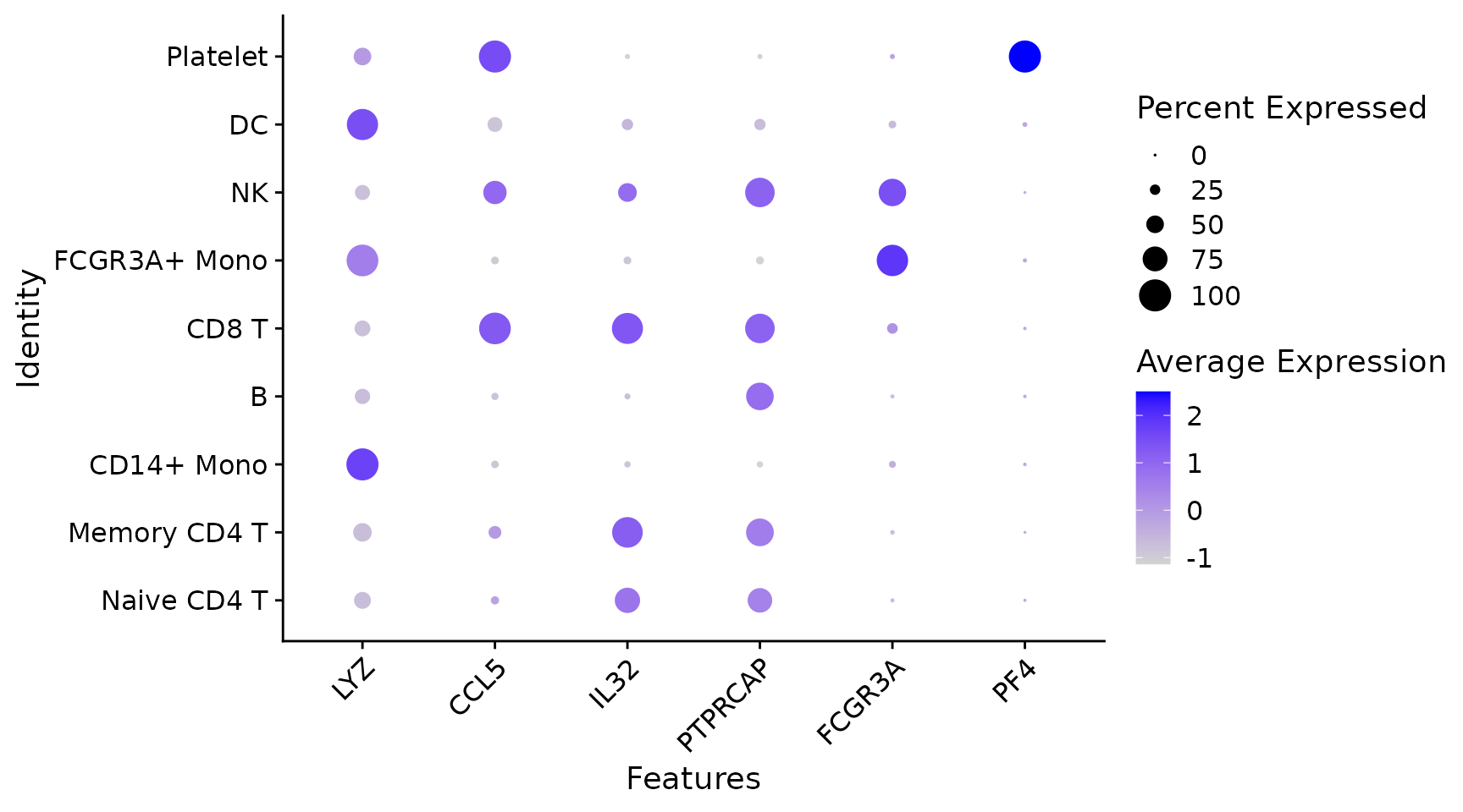
# Single cell heatmap of feature expression
DoHeatmap(subset(pbmc3k.final, downsample = 100), features = features, size = 3)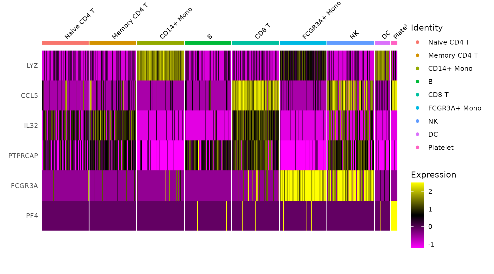
Customizing FeaturePlot
# Plot a legend to map colors to expression levels
FeaturePlot(pbmc3k.final, features = "MS4A1")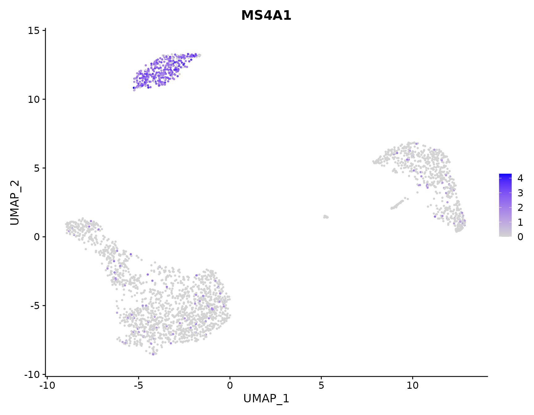
# Adjust the contrast in the plot
FeaturePlot(pbmc3k.final, features = "MS4A1", min.cutoff = 1, max.cutoff = 3)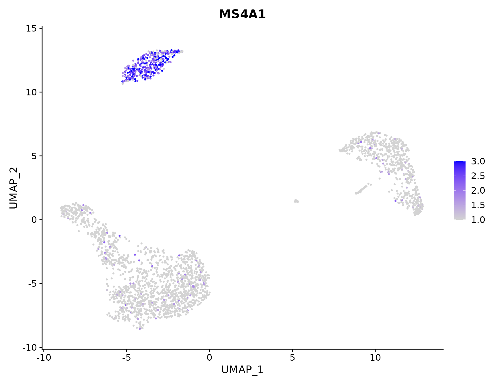
# Calculate feature-specific contrast levels based on quantiles of non-zero expression.
# Particularly useful when plotting multiple markers
FeaturePlot(pbmc3k.final, features = c("MS4A1", "PTPRCAP"), min.cutoff = "q10", max.cutoff = "q90")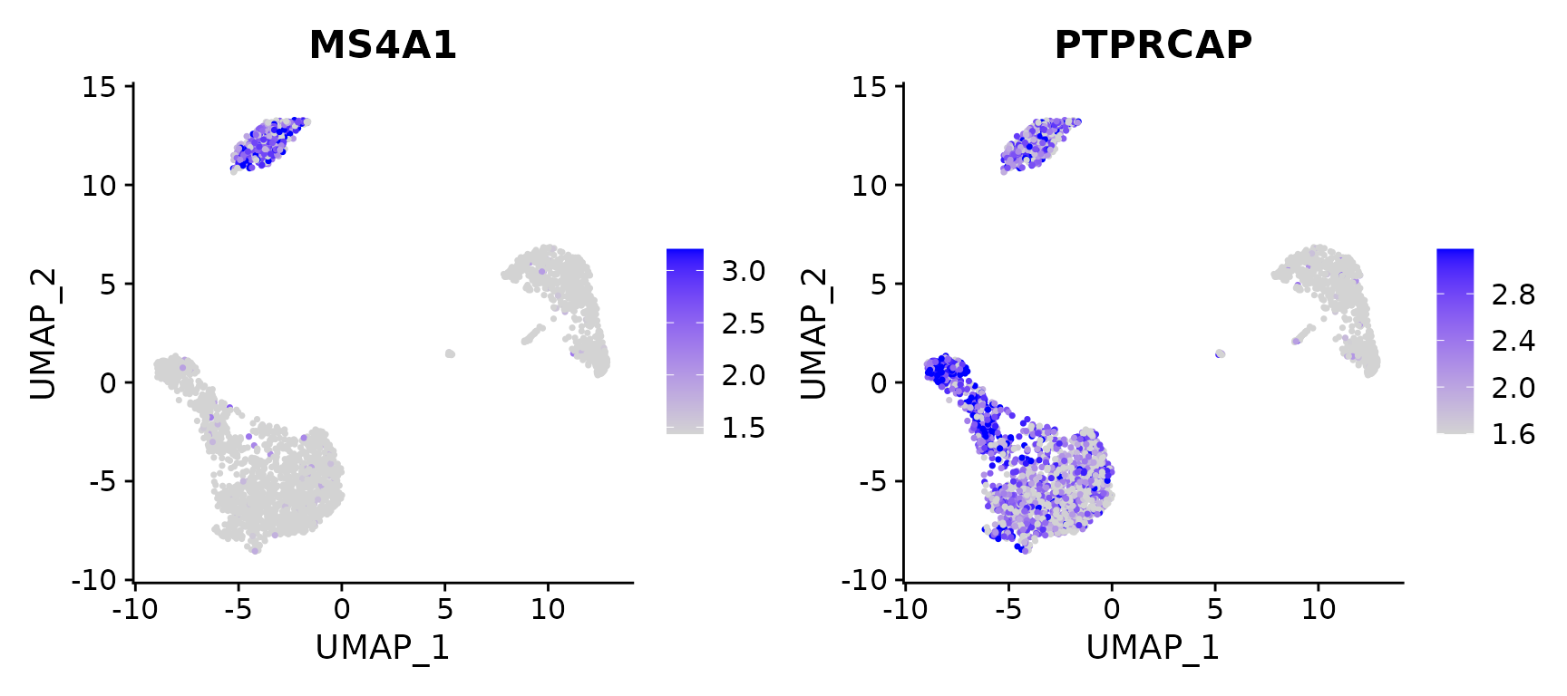
# Visualize co-expression of two features simultaneously
FeaturePlot(pbmc3k.final, features = c("MS4A1", "CD79A"), blend = TRUE)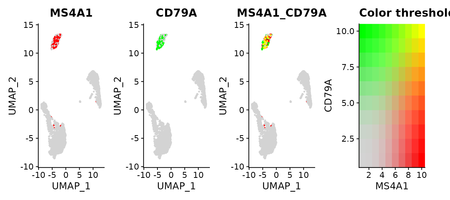
# Split visualization to view expression by groups (replaces FeatureHeatmap)
FeaturePlot(pbmc3k.final, features = c("MS4A1", "CD79A"), split.by = "groups")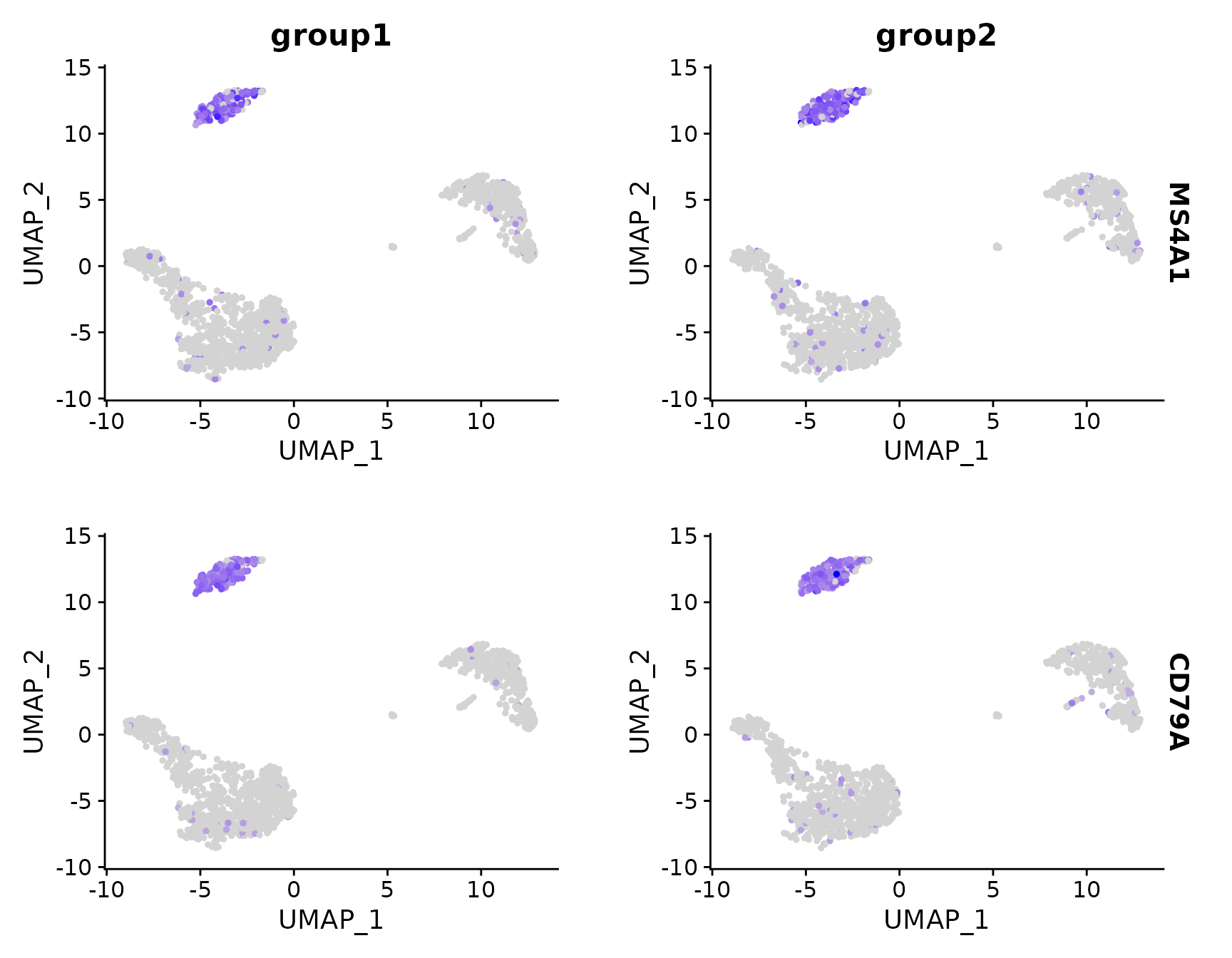
Other visualization functionality
# Violin plots can also be split on some variable. Simply add the splitting variable to object
# metadata and pass it to the split.by argument
VlnPlot(pbmc3k.final, features = "percent.mt", split.by = "groups")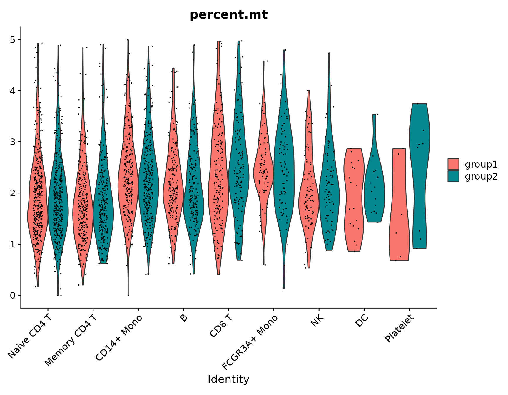
# SplitDotPlotGG is replaced with the `split.by` parameter for DotPlot
DotPlot(pbmc3k.final, features = features, split.by = "groups") + RotatedAxis()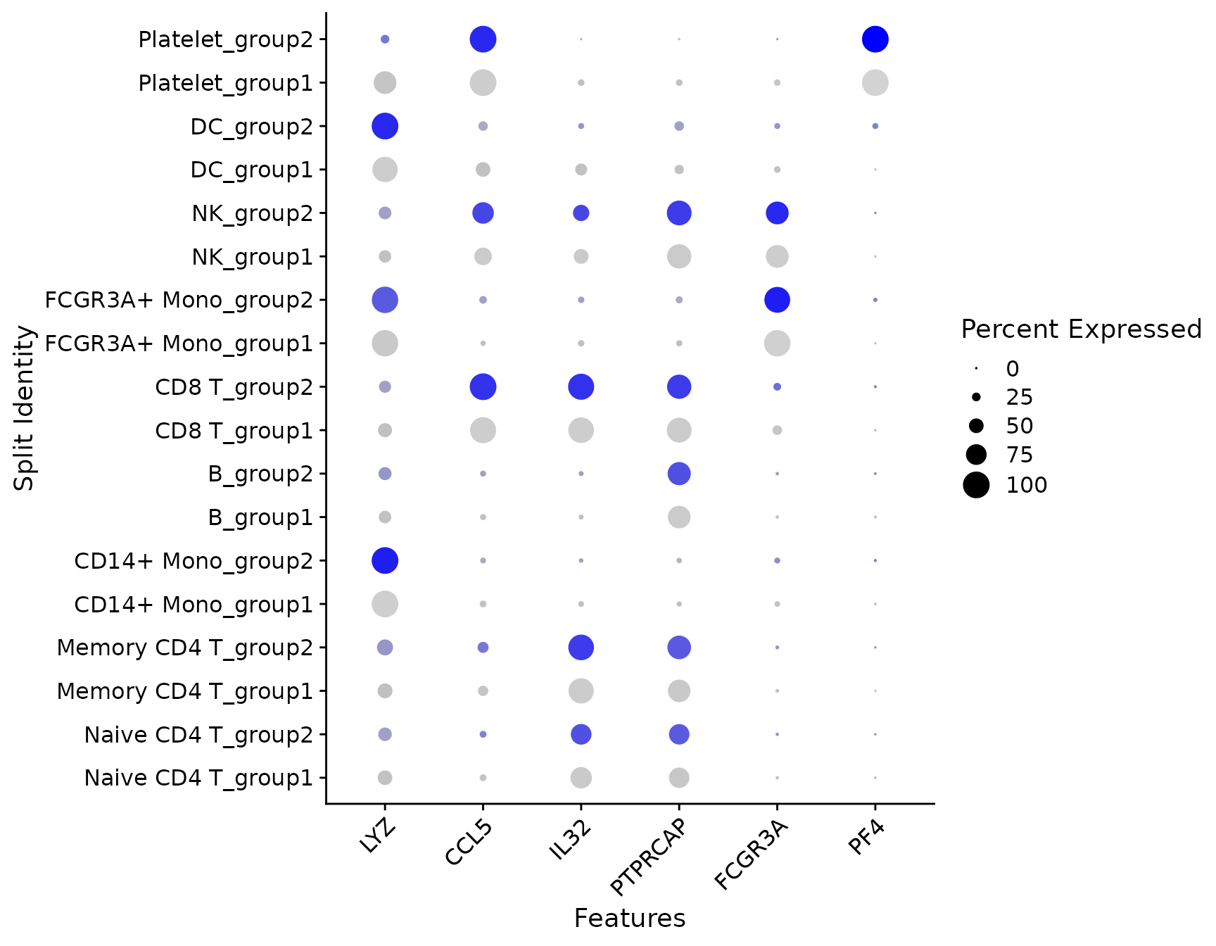
# DimPlot replaces TSNEPlot, PCAPlot, etc., and plots either 'umap', 'tsne', or 'pca' by
# default, in that order
DimPlot(pbmc3k.final)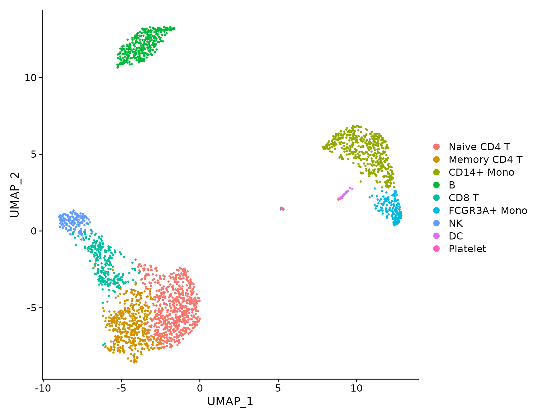
pbmc3k.final.no.umap <- pbmc3k.final
pbmc3k.final.no.umap[["umap"]] <- NULL
DimPlot(pbmc3k.final.no.umap) + RotatedAxis()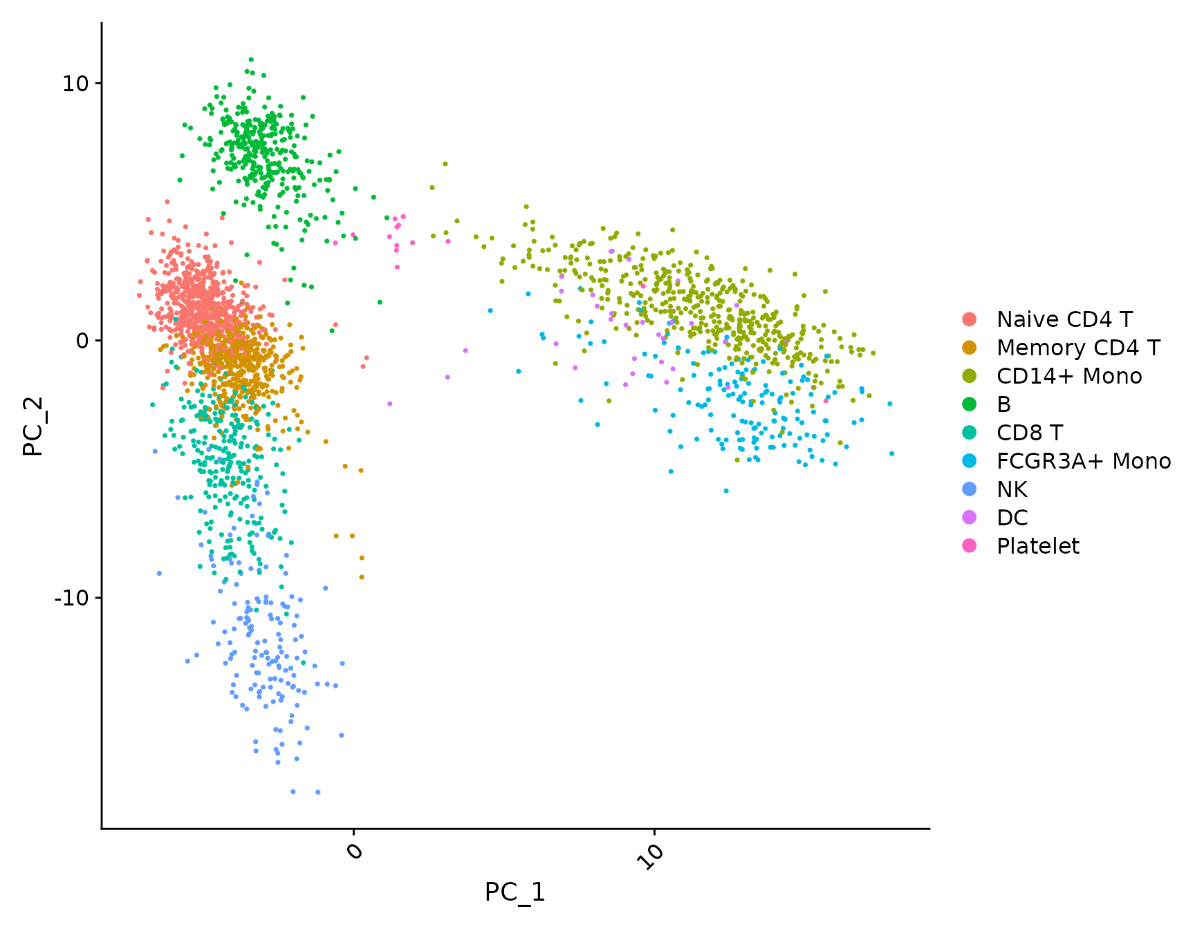
# DoHeatmap now shows a grouping bar, splitting the heatmap into groups or clusters. This can
# be changed with the `group.by` parameter
DoHeatmap(pbmc3k.final, features = VariableFeatures(pbmc3k.final)[1:100], cells = 1:500, size = 4,
    angle = 90) + NoLegend()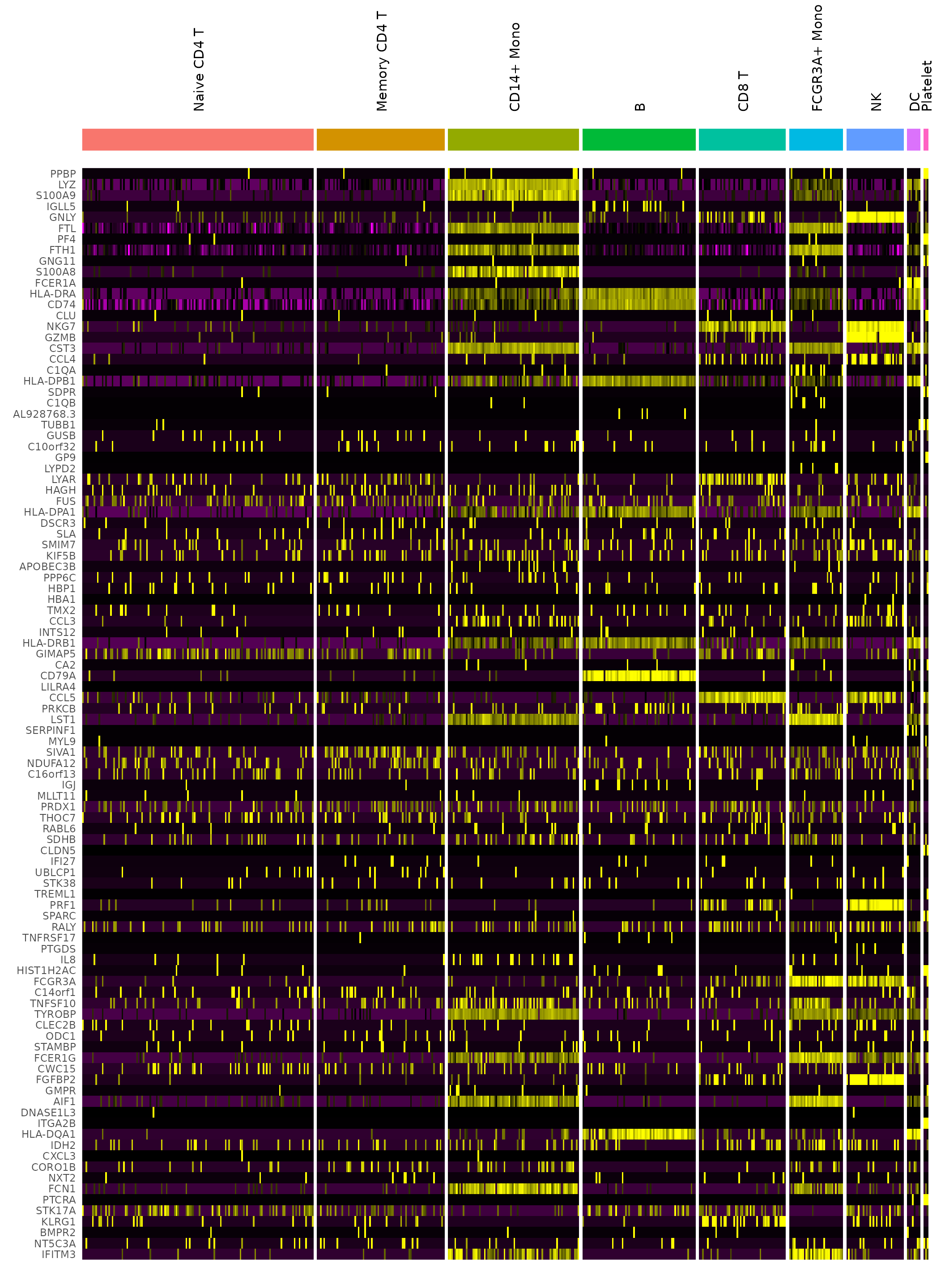
Applying themes to plots
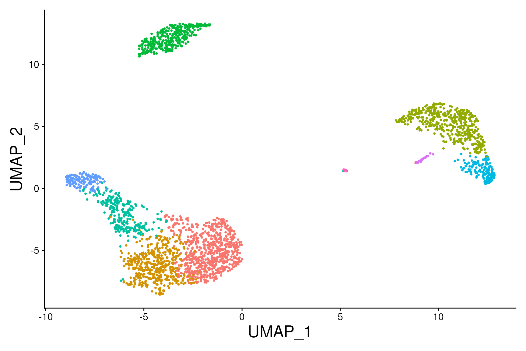
With Seurat, all plotting functions return plots as ggplot2 objects by default, allowing one to easily customize plots just like any other ggplot2-based plot.
baseplot <- DimPlot(pbmc3k.final, reduction = "umap")
# Add custom labels and titles
baseplot + labs(title = "Clustering of 2,700 PBMCs")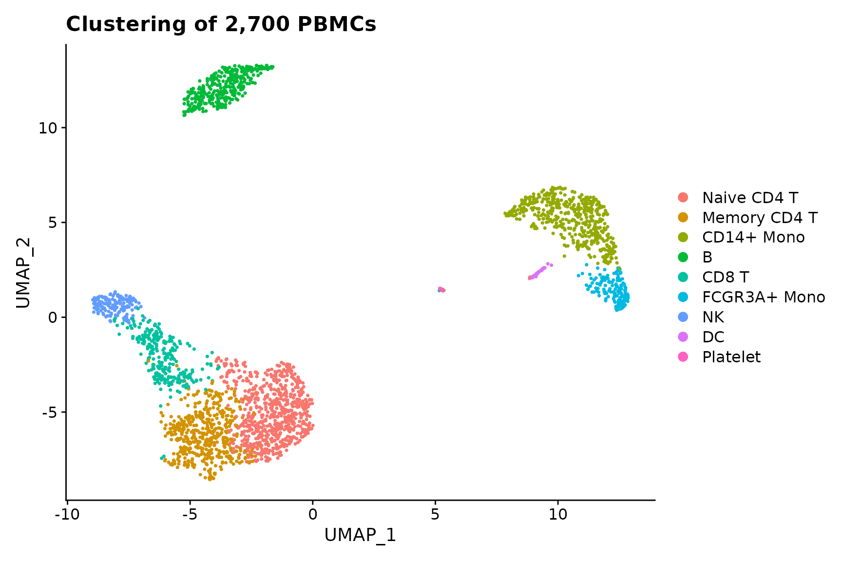
# Seurat also provides several built-in themes, such as DarkTheme; for more details see
# ?SeuratTheme
baseplot + DarkTheme()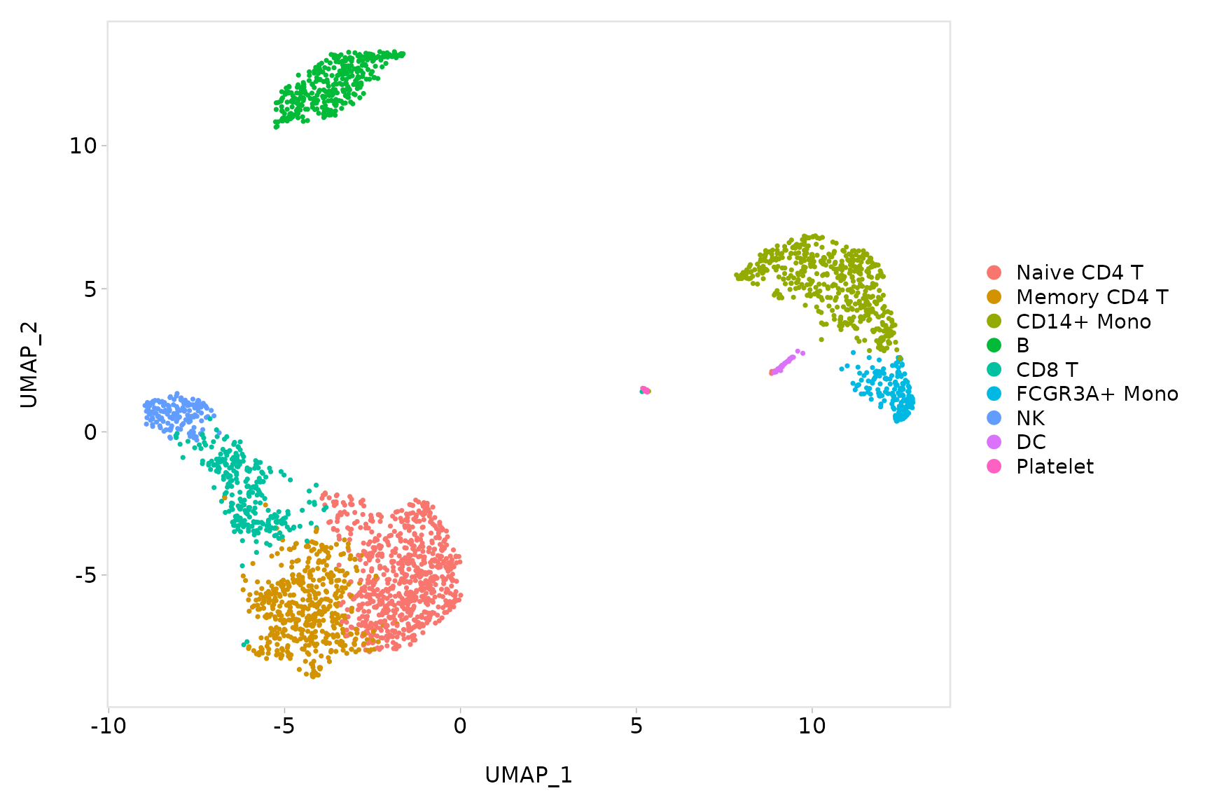
We can also chain themes together:
plot <- baseplot + DarkTheme() + theme(axis.title = element_text(size = 18), legend.text = element_text(size = 18)) +
    guides(colour = guide_legend(override.aes = list(size = 10)))

plot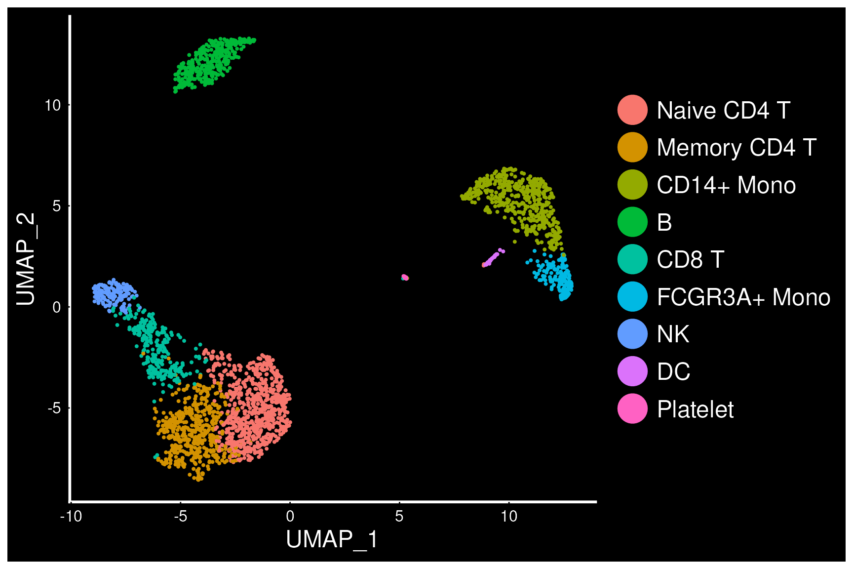
# ggsave(filename = '../output/images/visualization_vignette.jpg', height = 7, width = 12,
# plot = plot, quality = 50)
Interactive plotting features
Seurat utilizes R’s plotly graphing library to create
interactive plots. This interactive plotting feature works with any
ggplot2-based scatter plots (requires a geom_point layer).
To use, simply make a ggplot2-based scatter plot (such as
DimPlot() or FeaturePlot()) and pass the
resulting plot to HoverLocator()
# Include additional data to display alongside cell names by passing in a data frame of
# information.  Works well when using FetchData
plot <- FeaturePlot(pbmc3k.final, features = "MS4A1")
HoverLocator(plot = plot, information = FetchData(pbmc3k.final, vars = c("ident", "PC_1", "nFeature_RNA")))
Another interactive feature provided by Seurat is being able to
manually select cells for further investigation. We have found this
particularly useful for small clusters that do not always separate using
unbiased clustering, but which look tantalizingly distinct. You can now
select these cells by creating a ggplot2-based scatter plot (such as
with DimPlot() or FeaturePlot()), and passing
the returned plot to CellSelector().
CellSelector() will return a vector with the names of the
points selected, so that you can then set them to a new identity class
and perform differential expression.
For example, let’s pretend that DCs had merged with monocytes in the clustering, but we wanted to see what was unique about them based on their position in the tSNE plot.
pbmc3k.final <- RenameIdents(pbmc3k.final, DC = "CD14+ Mono")
plot <- DimPlot(pbmc3k.final, reduction = "umap")
select.cells <- CellSelector(plot = plot)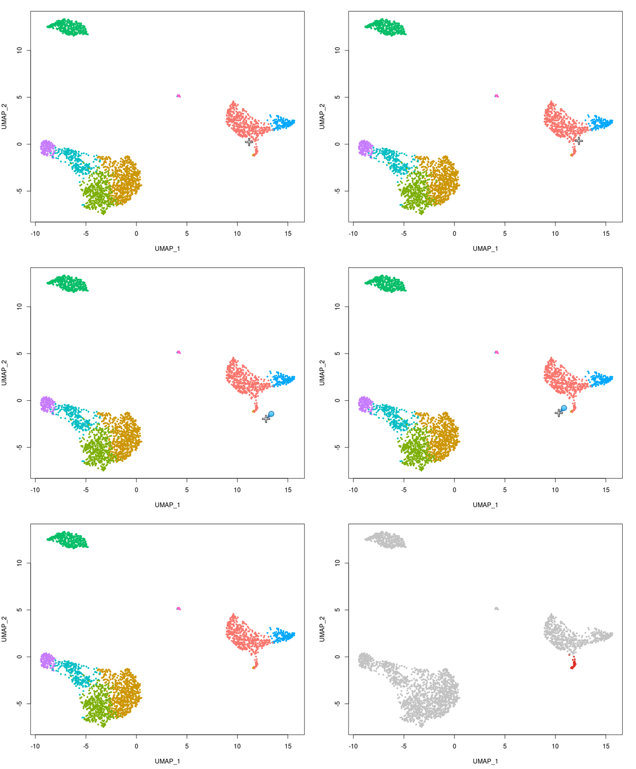
We can then change the identity of these cells to turn them into their own mini-cluster.
head(select.cells)## [1] "AAGATTACCGCCTT" "AAGCCATGAACTGC" "AATTACGAATTCCT" "ACCCGTTGCTTCTA"
## [5] "ACGAGGGACAGGAG" "ACGTGATGCCATGA"
Idents(pbmc3k.final, cells = select.cells) <- "NewCells"

# Now, we find markers that are specific to the new cells, and find clear DC markers
newcells.markers <- FindMarkers(pbmc3k.final, ident.1 = "NewCells", ident.2 = "CD14+ Mono", min.diff.pct = 0.3,
    only.pos = TRUE)
head(newcells.markers)
## p_val avg_log2FC pct.1 pct.2 p_val_adj
## FCER1A 3.239004e-69 6.504163 0.800 0.017 4.441970e-65
## SERPINF1 7.761413e-36 5.456560 0.457 0.013 1.064400e-31
## HLA-DQB2 1.721094e-34 4.752397 0.429 0.010 2.360309e-30
## CD1C 2.304106e-33 4.929607 0.514 0.025 3.159851e-29
## ENHO 5.099765e-32 5.076634 0.400 0.010 6.993818e-28
## ITM2C 4.299994e-29 5.660234 0.371 0.010 5.897012e-25
Using CellSelector to Automatically Assign Cell Identities
In addition to returning a vector of cell names,
CellSelector() can also take the selected cells and assign
a new identity to them, returning a Seurat object with the identity
classes already set. This is done by passing the Seurat object used to
make the plot into CellSelector(), as well as an identity
class. As an example, we’re going to select the same set of cells as
before, and set their identity class to “selected”
pbmc3k.final <- CellSelector(plot = plot, object = pbmc3k.final, ident = "selected")
levels(pbmc3k.final)## [1] "selected" "Naive CD4 T" "Memory CD4 T" "CD14+ Mono" "B"
## [6] "CD8 T" "FCGR3A+ Mono" "NK" "Platelet"Plotting Accessories
Seurat also provides accessory functions for manipulating and combining plots.
# LabelClusters and LabelPoints will label clusters (a coloring variable) or individual points
# on a ggplot2-based scatter plot
plot <- DimPlot(pbmc3k.final, reduction = "pca") + NoLegend()
LabelClusters(plot = plot, id = "ident")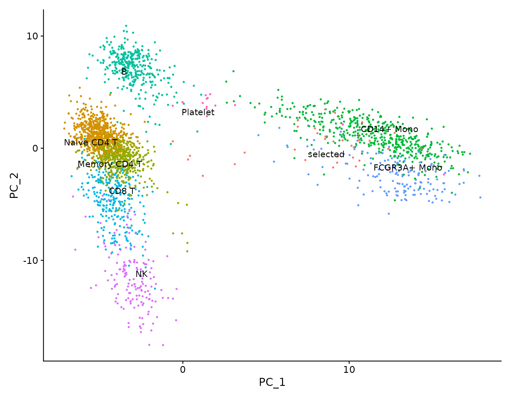
# Both functions support `repel`, which will intelligently stagger labels and draw connecting
# lines from the labels to the points or clusters
LabelPoints(plot = plot, points = TopCells(object = pbmc3k.final[["pca"]]), repel = TRUE)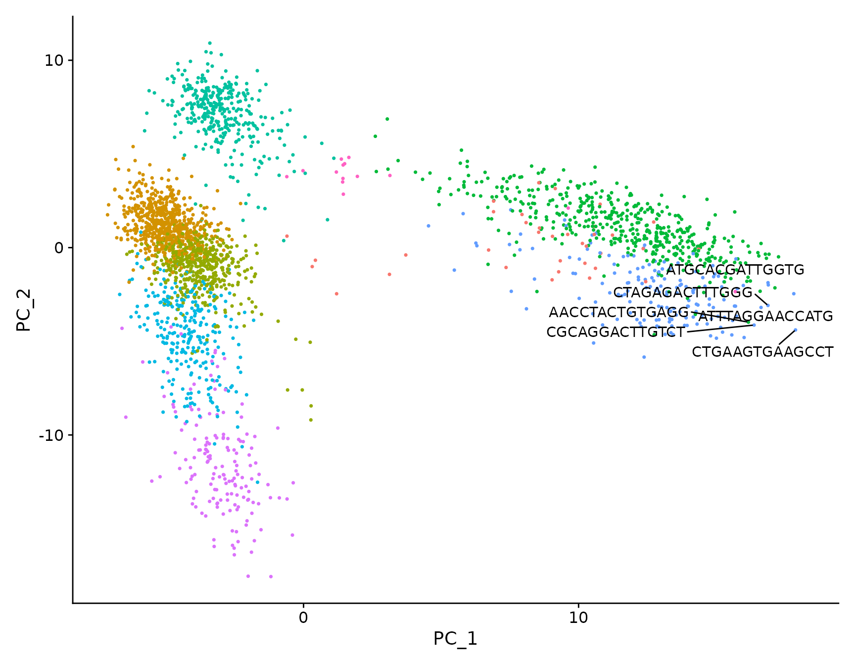
In early Seurat versions, we used the CombinePlots()
function to combine multiple plots together.
All plotting functions now use the patchwork system,
which allows for more flexible plot arrangements and easier
customization of combined plots; see the patchwork website for
more details and examples.
plot1 <- DimPlot(pbmc3k.final)
# Create scatter plot with the Pearson correlation value as the title
plot2 <- FeatureScatter(pbmc3k.final, feature1 = "LYZ", feature2 = "CCL5")
# Combine two plots
plot1 + plot2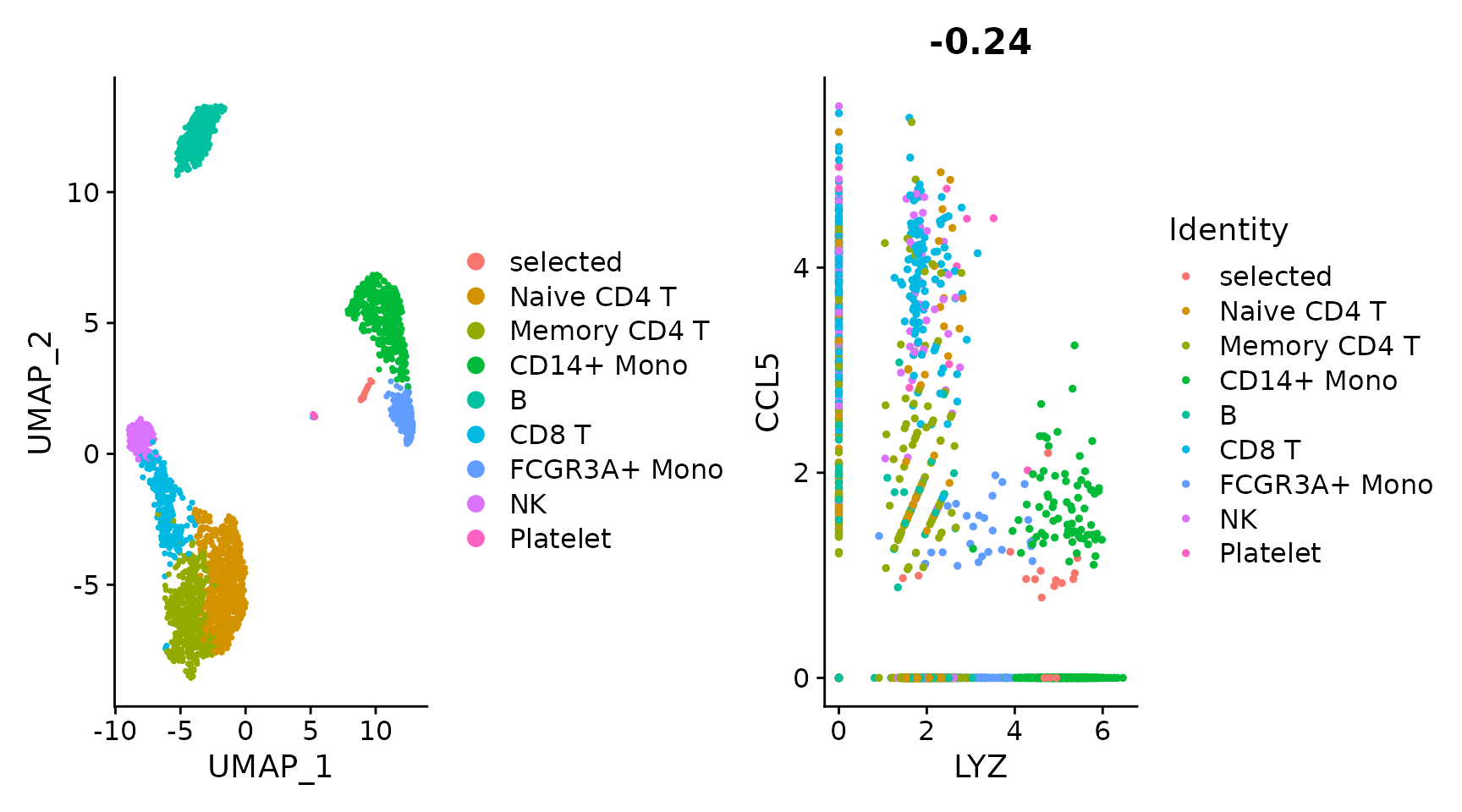
# Remove the legend from all plots
(plot1 + plot2) & NoLegend()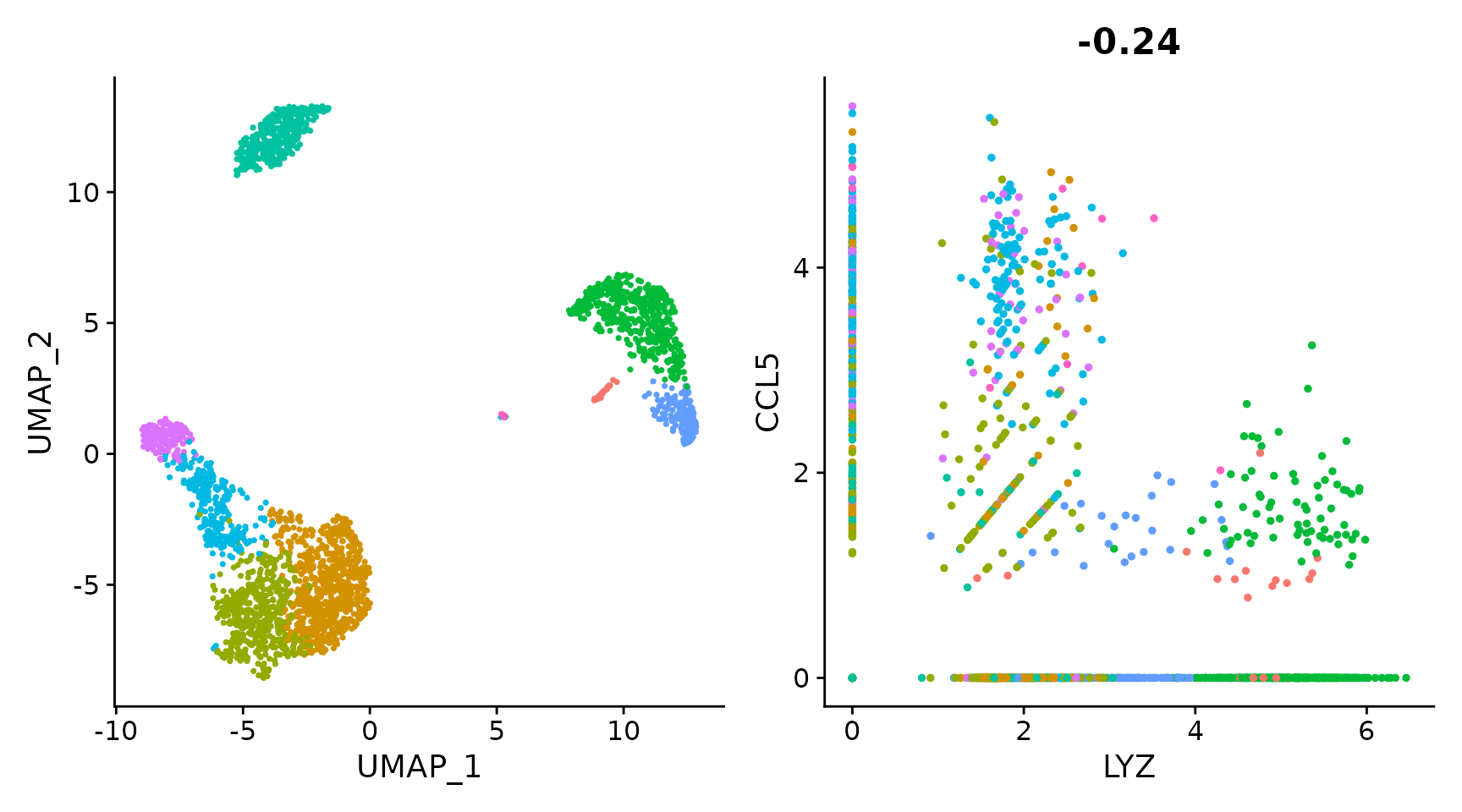
Session Info
## R version 4.5.2 (2025-10-31)
## Platform: x86_64-pc-linux-gnu
## Running under: Ubuntu 24.04.4 LTS
##
## Matrix products: default
## BLAS:   /usr/lib/x86_64-linux-gnu/openblas-pthread/libblas.so.3
## LAPACK: /usr/lib/x86_64-linux-gnu/openblas-pthread/libopenblasp-r0.3.26.so;  LAPACK version 3.12.0
##
## locale:
##  [1] LC_CTYPE=en_US.UTF-8       LC_NUMERIC=C
##  [3] LC_TIME=en_US.UTF-8        LC_COLLATE=en_US.UTF-8
##  [5] LC_MONETARY=en_US.UTF-8    LC_MESSAGES=en_US.UTF-8
##  [7] LC_PAPER=en_US.UTF-8       LC_NAME=C
##  [9] LC_ADDRESS=C               LC_TELEPHONE=C
## [11] LC_MEASUREMENT=en_US.UTF-8 LC_IDENTIFICATION=C
##
## time zone: Etc/UTC
## tzcode source: system (glibc)
##
## attached base packages:
## [1] stats     graphics  grDevices utils     datasets  methods   base
##
## other attached packages:
## [1] patchwork_1.3.2         ggplot2_4.0.3           pbmc3k.SeuratData_3.1.4
## [4] SeuratData_0.2.2.9002   Seurat_5.5.0            SeuratObject_5.4.0
## [7] sp_2.2-1
##
## loaded via a namespace (and not attached):
##   [1] RColorBrewer_1.1-3     jsonlite_2.0.0         magrittr_2.0.5
##   [4] spatstat.utils_3.2-2   ggbeeswarm_0.7.3       farver_2.1.2
##   [7] rmarkdown_2.30         fs_2.1.0               ragg_1.5.1
##  [10] vctrs_0.7.1            ROCR_1.0-12            spatstat.explore_3.8-0
##  [13] htmltools_0.5.9        sass_0.4.10            sctransform_0.4.3
##  [16] parallelly_1.47.0      KernSmooth_2.23-26     bslib_0.10.0
##  [19] htmlwidgets_1.6.4      desc_1.4.3             ica_1.0-3
##  [22] plyr_1.8.9             plotly_4.12.0          zoo_1.8-15
##  [25] cachem_1.1.0           igraph_2.3.0           mime_0.13
##  [28] lifecycle_1.0.5        pkgconfig_2.0.3        Matrix_1.7-5
##  [31] R6_2.6.1               fastmap_1.2.0          fitdistrplus_1.2-6
##  [34] future_1.70.0          shiny_1.13.0           digest_0.6.39
##  [37] tensor_1.5.1           RSpectra_0.16-2        irlba_2.3.7
##  [40] crosstalk_1.2.2        textshaping_1.0.5      labeling_0.4.3
##  [43] progressr_0.19.0       spatstat.sparse_3.1-0  httr_1.4.8
##  [46] polyclip_1.10-7        abind_1.4-8            compiler_4.5.2
##  [49] withr_3.0.2            S7_0.2.1               fastDummies_1.7.6
##  [52] MASS_7.3-65            rappdirs_0.3.4         tools_4.5.2
##  [55] vipor_0.4.7            lmtest_0.9-40          otel_0.2.0
##  [58] beeswarm_0.4.0         httpuv_1.6.16          future.apply_1.20.2
##  [61] goftest_1.2-3          glue_1.8.0             nlme_3.1-168
##  [64] promises_1.5.0         grid_4.5.2             Rtsne_0.17
##  [67] cluster_2.1.8.2        reshape2_1.4.5         generics_0.1.4
##  [70] gtable_0.3.6           spatstat.data_3.1-9    tidyr_1.3.2
##  [73] data.table_1.18.2.1    spatstat.geom_3.7-3    RcppAnnoy_0.0.23
##  [76] ggrepel_0.9.8          RANN_2.6.2             pillar_1.11.1
##  [79] stringr_1.6.0          limma_3.66.0           spam_2.11-3
##  [82] RcppHNSW_0.6.0         later_1.4.8            splines_4.5.2
##  [85] dplyr_1.2.0            lattice_0.22-7         survival_3.8-3
##  [88] deldir_2.0-4           tidyselect_1.2.1       miniUI_0.1.2
##  [91] pbapply_1.7-4          knitr_1.51             gridExtra_2.3
##  [94] scattermore_1.2        xfun_0.56              statmod_1.5.1
##  [97] matrixStats_1.5.0      stringi_1.8.7          lazyeval_0.2.3
## [100] yaml_2.3.12            evaluate_1.0.5         codetools_0.2-20
## [103] tibble_3.3.1           cli_3.6.6              uwot_0.2.4
## [106] xtable_1.8-8           reticulate_1.46.0      systemfonts_1.3.2
## [109] jquerylib_0.1.4        Rcpp_1.1.1-1.1         globals_0.19.1
## [112] spatstat.random_3.4-5  png_0.1-9              ggrastr_1.0.2
## [115] spatstat.univar_3.1-7  parallel_4.5.2         pkgdown_2.2.0
## [118] presto_1.0.0           dotCall64_1.2          listenv_0.10.1
## [121] viridisLite_0.4.3      scales_1.4.0           ggridges_0.5.7
## [124] purrr_1.2.1            crayon_1.5.3           rlang_1.2.0
## [127] cowplot_1.2.0          formatR_1.14