Mapping and annotating query datasets
Compiled: 2023-10-31
Source:vignettes/integration_mapping.Rmd
integration_mapping.RmdIntroduction to single-cell reference mapping
In this vignette, we first build an integrated reference and then demonstrate how to leverage this reference to annotate new query datasets. Generating an integrated reference follows the same workflow described in more detail in the integration introduction vignette. Once generated, this reference can be used to analyze additional query datasets through tasks like cell type label transfer and projecting query cells onto reference UMAPs. Notably, this does not require correction of the underlying raw query data and can therefore be an efficient strategy if a high quality reference is available.
Dataset preprocessing
For the purposes of this example, we’ve chosen human pancreatic islet cell datasets produced across four technologies, CelSeq (GSE81076) CelSeq2 (GSE85241), Fluidigm C1 (GSE86469), and SMART-Seq2 (E-MTAB-5061). For convenience, we distribute this dataset through our SeuratData package. The metadata contains the technology (tech column) and cell type annotations (celltype column) for each cell in the four datasets.
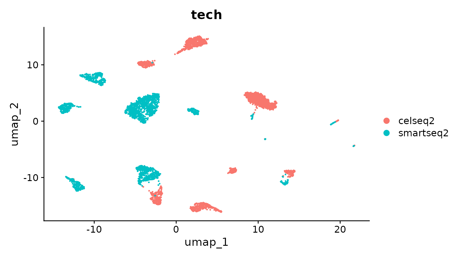
InstallData("panc8")As a demonstration, we will use a subset of technologies to construct a reference. We will then map the remaining datasets onto this reference. We start by selecting cells from four technologies, and performing an analysis without integration.
##
##     celseq    celseq2 fluidigmc1     indrop  smartseq2
##       1004       2285        638       8569       2394
# we will use data from 2 technologies for the reference
pancreas.ref <- subset(panc8, tech %in% c("celseq2", "smartseq2"))
pancreas.ref[["RNA"]] <- split(pancreas.ref[["RNA"]], f = pancreas.ref$tech)

# pre-process dataset (without integration)
pancreas.ref <- NormalizeData(pancreas.ref)
pancreas.ref <- FindVariableFeatures(pancreas.ref)
pancreas.ref <- ScaleData(pancreas.ref)
pancreas.ref <- RunPCA(pancreas.ref)
pancreas.ref <- FindNeighbors(pancreas.ref, dims = 1:30)
pancreas.ref <- FindClusters(pancreas.ref)
## Modularity Optimizer version 1.3.0 by Ludo Waltman and Nees Jan van Eck
##
## Number of nodes: 4679
## Number of edges: 174953
##
## Running Louvain algorithm...
## Maximum modularity in 10 random starts: 0.9180
## Number of communities: 19
## Elapsed time: 0 seconds
pancreas.ref <- RunUMAP(pancreas.ref, dims = 1:30)
DimPlot(pancreas.ref, group.by = c("celltytpe", "tech"))
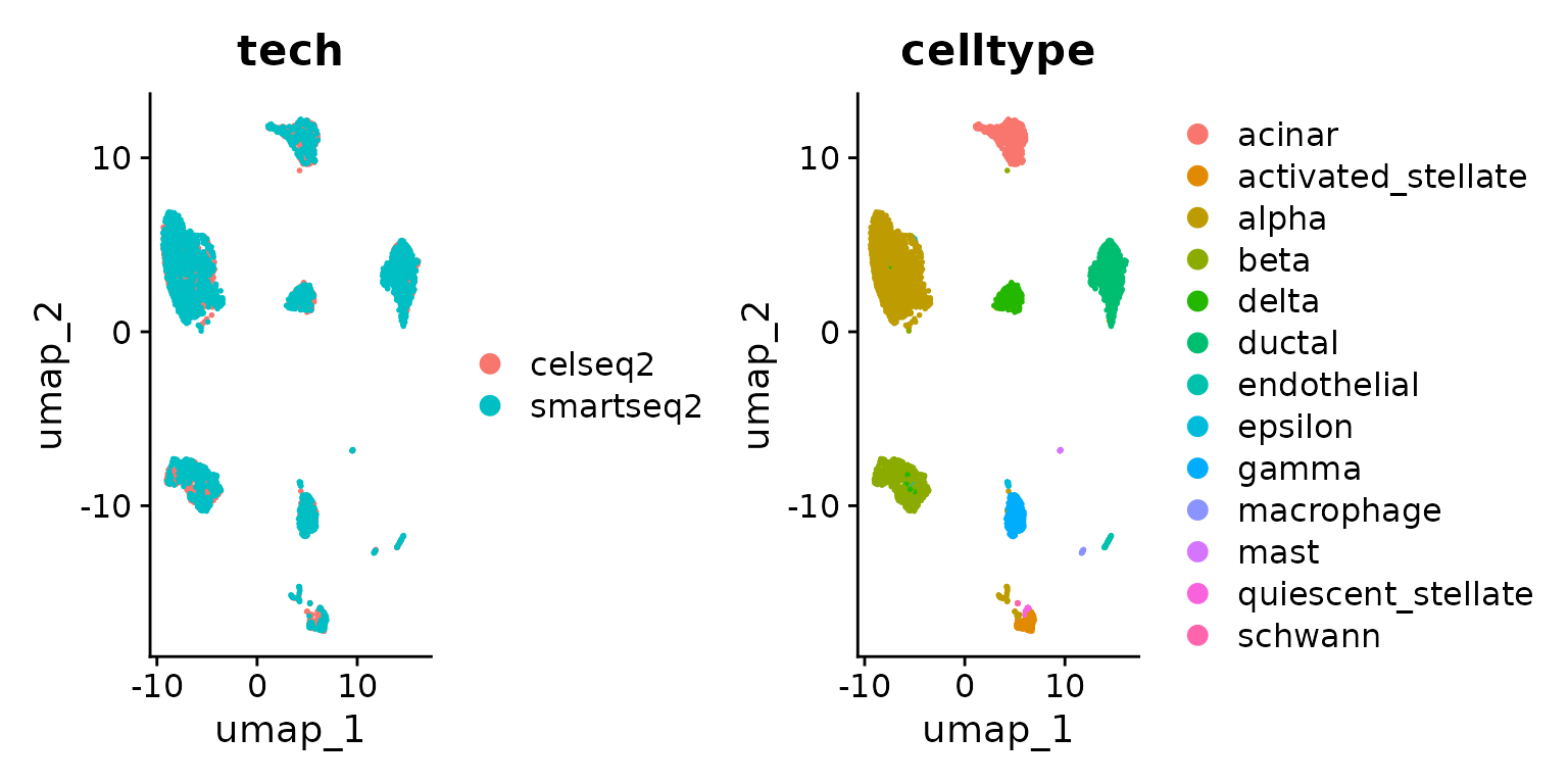
Next, we integrate the datasets into a shared reference. Please see our introduction to integration vignette
pancreas.ref <- IntegrateLayers(object = pancreas.ref, method = CCAIntegration, orig.reduction = "pca",
    new.reduction = "integrated.cca", verbose = FALSE)
pancreas.ref <- FindNeighbors(pancreas.ref, reduction = "integrated.cca", dims = 1:30)
pancreas.ref <- FindClusters(pancreas.ref)
## Modularity Optimizer version 1.3.0 by Ludo Waltman and Nees Jan van Eck
##
## Number of nodes: 4679
## Number of edges: 190152
##
## Running Louvain algorithm...
## Maximum modularity in 10 random starts: 0.8680
## Number of communities: 15
## Elapsed time: 0 seconds
pancreas.ref <- RunUMAP(pancreas.ref, reduction = "integrated.cca", dims = 1:30)
DimPlot(pancreas.ref, group.by = c("tech", "celltype"))
Cell type classification using an integrated reference
Seurat also supports the projection of reference data (or meta data) onto a query object. While many of the methods are conserved (both procedures begin by identifying anchors), there are two important distinctions between data transfer and integration:
- In data transfer, Seurat does not correct or modify the query expression data.
- In data transfer, Seurat has an option (set by default) to project the PCA structure of a reference onto the query, instead of learning a joint structure with CCA. We generally suggest using this option when projecting data between scRNA-seq datasets.
After finding anchors, we use the TransferData() function to classify the query cells based on reference data (a vector of reference cell type labels). TransferData() returns a matrix with predicted IDs and prediction scores, which we can add to the query metadata.
# select two technologies for the query datasets
pancreas.query <- subset(panc8, tech %in% c("fluidigmc1", "celseq"))
pancreas.query <- NormalizeData(pancreas.query)
pancreas.anchors <- FindTransferAnchors(reference = pancreas.ref, query = pancreas.query, dims = 1:30,
    reference.reduction = "pca")
predictions <- TransferData(anchorset = pancreas.anchors, refdata = pancreas.ref$celltype, dims = 1:30)
pancreas.query <- AddMetaData(pancreas.query, metadata = predictions)
Because we have the original label annotations from our full integrated analysis, we can evaluate how well our predicted cell type annotations match the full reference. In this example, we find that there is a high agreement in cell type classification, with over 96% of cells being labeled correctly.
pancreas.query$prediction.match <- pancreas.query$predicted.id == pancreas.query$celltype
table(pancreas.query$prediction.match)
##
## FALSE TRUE
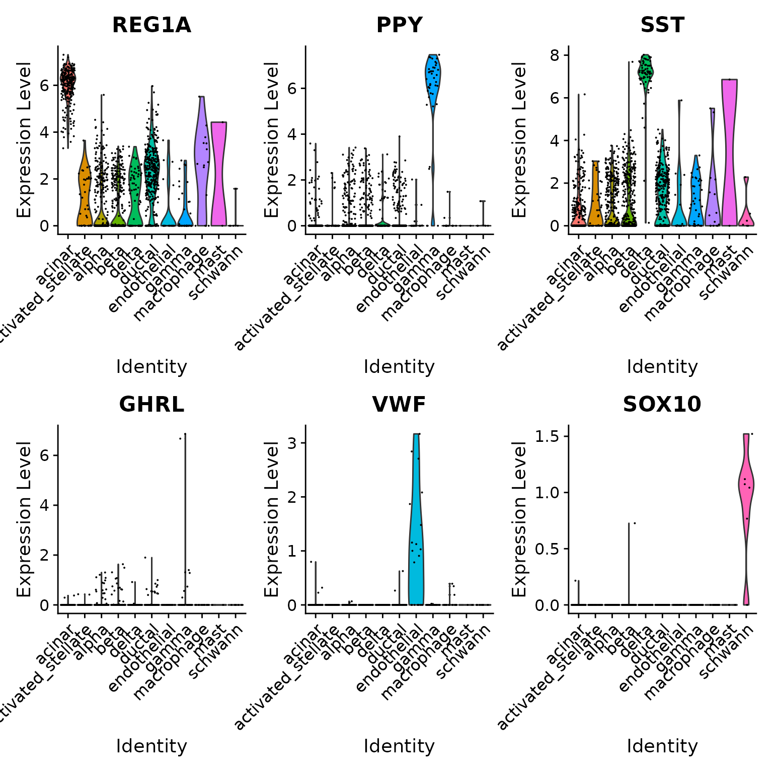
## 63 1579To verify this further, we can examine some canonical cell type markers for specific pancreatic islet cell populations. Note that even though some of these cell types are only represented by one or two cells (e.g. epsilon cells), we are still able to classify them correctly.
table(pancreas.query$predicted.id)##
## acinar activated_stellate alpha beta
## 262 39 436 419
## delta ductal endothelial gamma
## 73 330 19 41
## macrophage mast schwann
## 15 2 6
VlnPlot(pancreas.query, c("REG1A", "PPY", "SST", "GHRL", "VWF", "SOX10"), group.by = "predicted.id")
Unimodal UMAP Projection
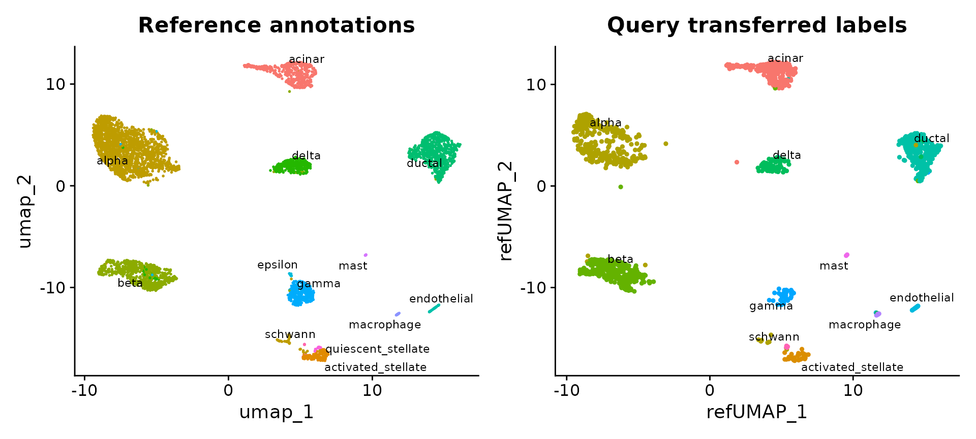
We also enable projection of a query onto the reference UMAP structure. This can be achieved by computing the reference UMAP model and then calling MapQuery() instead of TransferData().
pancreas.ref <- RunUMAP(pancreas.ref, dims = 1:30, reduction = "integrated.cca", return.model = TRUE)
pancreas.query <- MapQuery(anchorset = pancreas.anchors, reference = pancreas.ref, query = pancreas.query,
    refdata = list(celltype = "celltype"), reference.reduction = "pca", reduction.model = "umap")
What is
MapQuery doing?
MapQuery() is a wrapper around three functions: TransferData(), IntegrateEmbeddings(), and ProjectUMAP(). TransferData() is used to transfer cell type labels and impute the ADT values; IntegrateEmbeddings() is used to integrate reference with query by correcting the query’s projected low-dimensional embeddings; and finally ProjectUMAP() is used to project the query data onto the UMAP structure of the reference. The equivalent code for doing this with the intermediate functions is below:
pancreas.query <- TransferData(anchorset = pancreas.anchors, reference = pancreas.ref, query = pancreas.query,
    refdata = list(celltype = "celltype"))
pancreas.query <- IntegrateEmbeddings(anchorset = pancreas.anchors, reference = pancreas.ref, query = pancreas.query,
    new.reduction.name = "ref.pca")
pancreas.query <- ProjectUMAP(query = pancreas.query, query.reduction = "ref.pca", reference = pancreas.ref,
    reference.reduction = "pca", reduction.model = "umap")
We can now visualize the query cells alongside our reference.
p1 <- DimPlot(pancreas.ref, reduction = "umap", group.by = "celltype", label = TRUE, label.size = 3,
    repel = TRUE) + NoLegend() + ggtitle("Reference annotations")
p2 <- DimPlot(pancreas.query, reduction = "ref.umap", group.by = "predicted.celltype", label = TRUE,
    label.size = 3, repel = TRUE) + NoLegend() + ggtitle("Query transferred labels")
p1 + p2
Session Info
## R version 4.2.2 Patched (2022-11-10 r83330)
## Platform: x86_64-pc-linux-gnu (64-bit)
## Running under: Ubuntu 20.04.6 LTS
##
## Matrix products: default
## BLAS:   /usr/lib/x86_64-linux-gnu/blas/libblas.so.3.9.0
## LAPACK: /usr/lib/x86_64-linux-gnu/lapack/liblapack.so.3.9.0
##
## locale:
##  [1] LC_CTYPE=en_US.UTF-8       LC_NUMERIC=C
##  [3] LC_TIME=en_US.UTF-8        LC_COLLATE=en_US.UTF-8
##  [5] LC_MONETARY=en_US.UTF-8    LC_MESSAGES=en_US.UTF-8
##  [7] LC_PAPER=en_US.UTF-8       LC_NAME=C
##  [9] LC_ADDRESS=C               LC_TELEPHONE=C
## [11] LC_MEASUREMENT=en_US.UTF-8 LC_IDENTIFICATION=C
##
## attached base packages:
## [1] stats     graphics  grDevices utils     datasets  methods   base
##
## other attached packages:
##  [1] ggplot2_3.4.4                 thp1.eccite.SeuratData_3.1.5
##  [3] stxBrain.SeuratData_0.1.1     ssHippo.SeuratData_3.1.4
##  [5] pbmcsca.SeuratData_3.0.0      pbmcref.SeuratData_1.0.0
##  [7] pbmcMultiome.SeuratData_0.1.4 pbmc3k.SeuratData_3.1.4
##  [9] panc8.SeuratData_3.0.2        ifnb.SeuratData_3.0.0
## [11] hcabm40k.SeuratData_3.0.0     cbmc.SeuratData_3.1.4
## [13] bmcite.SeuratData_0.3.0       SeuratData_0.2.2.9001
## [15] Seurat_5.0.0                  SeuratObject_5.0.0
## [17] sp_2.1-1
##
## loaded via a namespace (and not attached):
##   [1] spam_2.10-0            systemfonts_1.0.4      plyr_1.8.9
##   [4] igraph_1.5.1           lazyeval_0.2.2         splines_4.2.2
##   [7] RcppHNSW_0.5.0         listenv_0.9.0          scattermore_1.2
##  [10] digest_0.6.33          htmltools_0.5.6.1      fansi_1.0.5
##  [13] magrittr_2.0.3         memoise_2.0.1          tensor_1.5
##  [16] cluster_2.1.4          ROCR_1.0-11            globals_0.16.2
##  [19] matrixStats_1.0.0      pkgdown_2.0.7          spatstat.sparse_3.0-3
##  [22] colorspace_2.1-0       rappdirs_0.3.3         ggrepel_0.9.4
##  [25] textshaping_0.3.6      xfun_0.40              dplyr_1.1.3
##  [28] crayon_1.5.2           jsonlite_1.8.7         progressr_0.14.0
##  [31] spatstat.data_3.0-3    survival_3.5-7         zoo_1.8-12
##  [34] glue_1.6.2             polyclip_1.10-6        gtable_0.3.4
##  [37] leiden_0.4.3           future.apply_1.11.0    abind_1.4-5
##  [40] scales_1.2.1           spatstat.random_3.2-1  miniUI_0.1.1.1
##  [43] Rcpp_1.0.11            viridisLite_0.4.2      xtable_1.8-4
##  [46] reticulate_1.34.0      dotCall64_1.1-0        htmlwidgets_1.6.2
##  [49] httr_1.4.7             RColorBrewer_1.1-3     ellipsis_0.3.2
##  [52] ica_1.0-3              farver_2.1.1           pkgconfig_2.0.3
##  [55] sass_0.4.7             uwot_0.1.16            deldir_1.0-9
##  [58] utf8_1.2.4             labeling_0.4.3         tidyselect_1.2.0
##  [61] rlang_1.1.1            reshape2_1.4.4         later_1.3.1
##  [64] munsell_0.5.0          tools_4.2.2            cachem_1.0.8
##  [67] cli_3.6.1              generics_0.1.3         ggridges_0.5.4
##  [70] evaluate_0.22          stringr_1.5.0          fastmap_1.1.1
##  [73] yaml_2.3.7             ragg_1.2.5             goftest_1.2-3
##  [76] knitr_1.45             fs_1.6.3               fitdistrplus_1.1-11
##  [79] purrr_1.0.2            RANN_2.6.1             pbapply_1.7-2
##  [82] future_1.33.0          nlme_3.1-162           mime_0.12
##  [85] formatR_1.14           ggrastr_1.0.1          compiler_4.2.2
##  [88] beeswarm_0.4.0         plotly_4.10.3          png_0.1-8
##  [91] spatstat.utils_3.0-4   tibble_3.2.1           bslib_0.5.1
##  [94] stringi_1.7.12         highr_0.10             desc_1.4.2
##  [97] RSpectra_0.16-1        lattice_0.21-9         Matrix_1.6-1.1
## [100] vctrs_0.6.4            pillar_1.9.0           lifecycle_1.0.3
## [103] spatstat.geom_3.2-7    lmtest_0.9-40          jquerylib_0.1.4
## [106] RcppAnnoy_0.0.21       data.table_1.14.8      cowplot_1.1.1
## [109] irlba_2.3.5.1          httpuv_1.6.12          patchwork_1.1.3
## [112] R6_2.5.1               promises_1.2.1         KernSmooth_2.23-22
## [115] gridExtra_2.3          vipor_0.4.5            parallelly_1.36.0
## [118] codetools_0.2-19       fastDummies_1.7.3      MASS_7.3-58.2
## [121] rprojroot_2.0.3        withr_2.5.2            sctransform_0.4.1
## [124] parallel_4.2.2         grid_4.2.2             tidyr_1.3.0
## [127] rmarkdown_2.25         Rtsne_0.16             spatstat.explore_3.2-5
## [130] shiny_1.7.5.1          ggbeeswarm_0.7.1