Using sctransform in Seurat
Saket Choudhary, Christoph Hafemeister & Rahul Satija
Compiled: April 28, 2026
Source:vignettes/sctransform_vignette.Rmd
sctransform_vignette.RmdBiological heterogeneity in single-cell RNA-seq data is often confounded by technical factors including sequencing depth. The number of molecules detected in each cell can vary significantly between cells, even within the same celltype. Interpretation of scRNA-seq data requires effective pre-processing and normalization to remove this technical variability.
In Hafemeister
and Satija, 2019, we introduced a modeling framework,
sctransform, for the normalization and variance
stabilization of molecular count data from scRNA-seq experiments. This
procedure omits the need for heuristic steps including pseudocount
addition or log-transformation and improves common downstream analytical
tasks such as variable gene selection, dimensional reduction, and
differential expression.
Inspired by important and rigorous work from Lause
et al, we released an updated
manuscript and updated the sctransform software to
version v2, which is now the default in Seurat v5.
Load data and create Seurat object
pbmc_data <- Read10X(data.dir = "/brahms/shared/vignette-data/pbmc3k/filtered_gene_bc_matrices/hg19/")
pbmc <- CreateSeuratObject(counts = pbmc_data)
Apply sctransform normalization
The single command SCTransform() replaces
NormalizeData(), ScaleData(), and
FindVariableFeatures(). The glmGamPoi package
substantially improves speed and is used by default if installed.
In Seurat v5, SCT v2 is applied by default. You can revert to v1 by
setting vst.flavor = 'v1'. During normalization, we can
also remove confounding sources of variation, for example, mitochondrial
mapping percentage.
After running SCTransform(), transformed data is
available in the “SCT” assay, which is set as the default assay. This
means that all downstream commands will use the sctransform-normalized
data by default.
# store mitochondrial percentage in object meta data
pbmc <- PercentageFeatureSet(pbmc, pattern = "^MT-", col.name = 'percent.mt')

# run sctransform
pbmc <- SCTransform(pbmc, vars.to.regress = "percent.mt", verbose = FALSE)
Perform dimensionality reduction by PCA and UMAP embedding
# These are now standard steps in the Seurat workflow for visualization and clustering
pbmc <- RunPCA(pbmc, verbose = FALSE)
pbmc <- RunUMAP(pbmc, dims = 1:30, verbose = FALSE)

pbmc <- FindNeighbors(pbmc, dims = 1:30, verbose = FALSE)
pbmc <- FindClusters(pbmc, verbose = FALSE)

DimPlot(pbmc, label = TRUE) 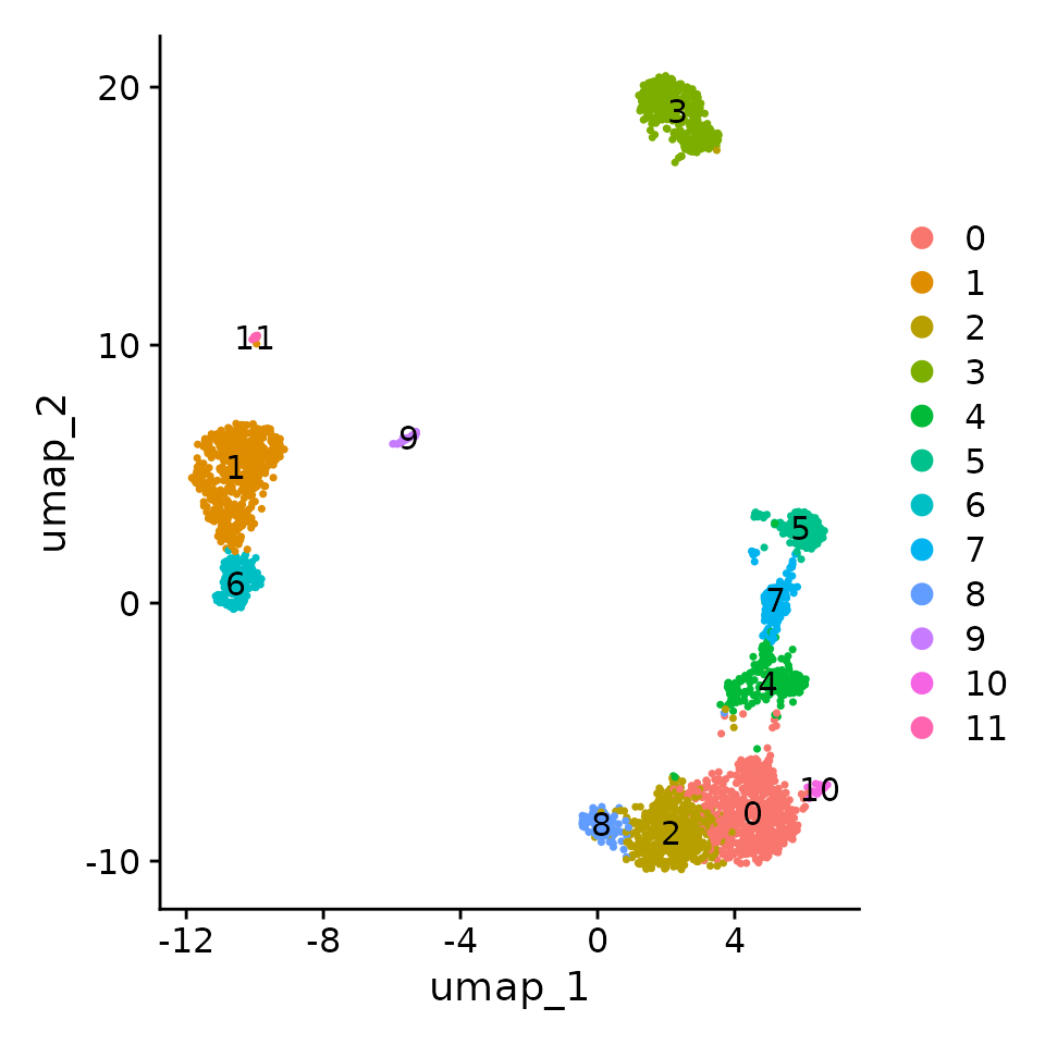
Why can we choose more PCs when using sctransform?
In the standard Seurat workflow, we focus on 10 PCs for this dataset, though we highlight that the results are similar with higher settings for this parameter. Interestingly, we’ve found that when using sctransform, we often benefit by pushing this parameter even higher. We believe this is because the sctransform workflow performs more effective normalization, strongly removing technical effects from the data.
Even after standard log-normalization, variation in sequencing depth is still a confounding factor (see Figure 1), and this effect can subtly influence higher PCs. In sctransform, this effect is substantially mitigated (see Figure 3). This means that higher PCs are more likely to represent subtle, but biologically relevant, sources of heterogeneity – so including them may improve downstream analysis.
In addition, sctransform returns 3,000 variable features by default, instead of 2,000. The rationale is similar, the additional variable features are less likely to be driven by technical differences across cells, and instead may represent more subtle biological fluctuations. In general, we find that results produced with sctransform are less dependent on these parameters (indeed, we achieve nearly identical results when using all genes in the transcriptome, though this does reduce computational efficiency). This can help users generate more robust results, and in addition, enables the application of standard analysis pipelines with identical parameter settings that can quickly be applied to new datasets:
For example, the following code replicates the full end-to-end workflow, in a single command:
library(dplyr)
pbmc <- CreateSeuratObject(pbmc_data) %>%
          PercentageFeatureSet(pattern = "^MT-",col.name = 'percent.mt') %>%
          SCTransform(vars.to.regress = 'percent.mt') %>%
          RunPCA() %>%
          FindNeighbors(dims = 1:30) %>%
          RunUMAP(dims = 1:30) %>%
          FindClusters()
Where are normalized values stored for sctransform?
The results of sctransform are stored in the “SCT” assay. You can learn more about multi-assay data and commands in Seurat in our vignette, command cheat sheet, and SeuratObject documentation.
-
pbmc[["SCT"]]$scale.datacontains the residuals (normalized values), and is used directly as input to PCA. Please note that this matrix is non-sparse, and can therefore take up a lot of memory if stored for all genes. To save memory, we store these values only for variable genes, by settingreturn.only.var.genes = TRUEby default in the call toSCTransform(). - To assist with visualization and interpretation, we also convert
Pearson residuals back to ‘corrected’ UMI counts. You can interpret
these as the UMI counts we would expect to observe if all cells were
sequenced to the same depth. If you want to see exactly how we do this,
please look at the
correctfunction here. - The ‘corrected’ UMI counts are stored in
pbmc[["SCT"]]$counts. We store log-normalized versions of these corrected counts inpbmc[["SCT"]]$data, which are very helpful for visualization.
Users can individually annotate clusters based on canonical markers. However, the sctransform normalization reveals sharper biological distinctions compared to the standard Seurat workflow, in a few ways:
- Clear separation of at least 3 CD8 T cell populations (naive, memory, effector), based on CD8A, GZMK, CCL5, CCR7 expression
- Clear separation of three CD4 T cell populations (naive, memory, IFN-activated) based on S100A4, CCR7, IL32, and ISG15
- Additional developmental sub-structure in B cell cluster, based on TCL1A, FCER2
- Additional separation of NK cells into CD56dim vs. bright clusters, based on XCL1 and FCGR3A
# These are now standard steps in the Seurat workflow for visualization and clustering
# Visualize canonical marker genes as violin plots.
VlnPlot(pbmc, features = c("CD8A", "GZMK", "CCL5", "S100A4", "ANXA1", "CCR7", "ISG15", "CD3D"), pt.size = 0.2, ncol = 4)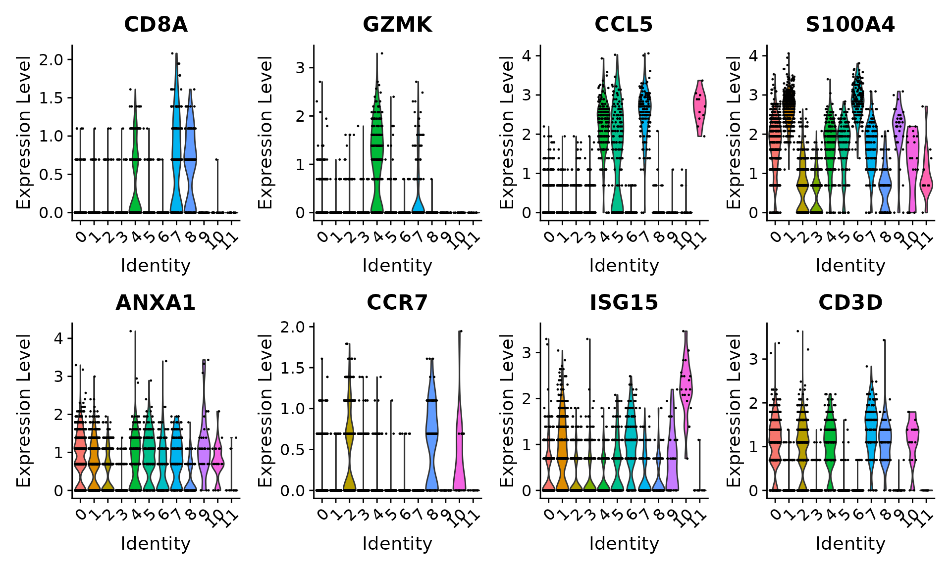
# Visualize canonical marker genes on the sctransform embedding.
FeaturePlot(pbmc, features = c("CD8A", "GZMK", "CCL5", "S100A4", "ANXA1", "CCR7"), pt.size = 0.2, ncol = 3)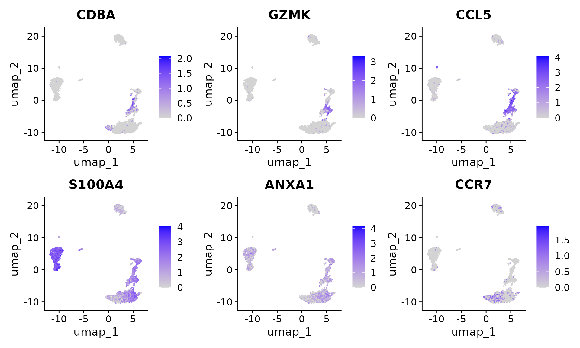
FeaturePlot(pbmc, features = c("CD3D", "ISG15", "TCL1A", "FCER2", "XCL1", "FCGR3A"), pt.size = 0.2, ncol = 3)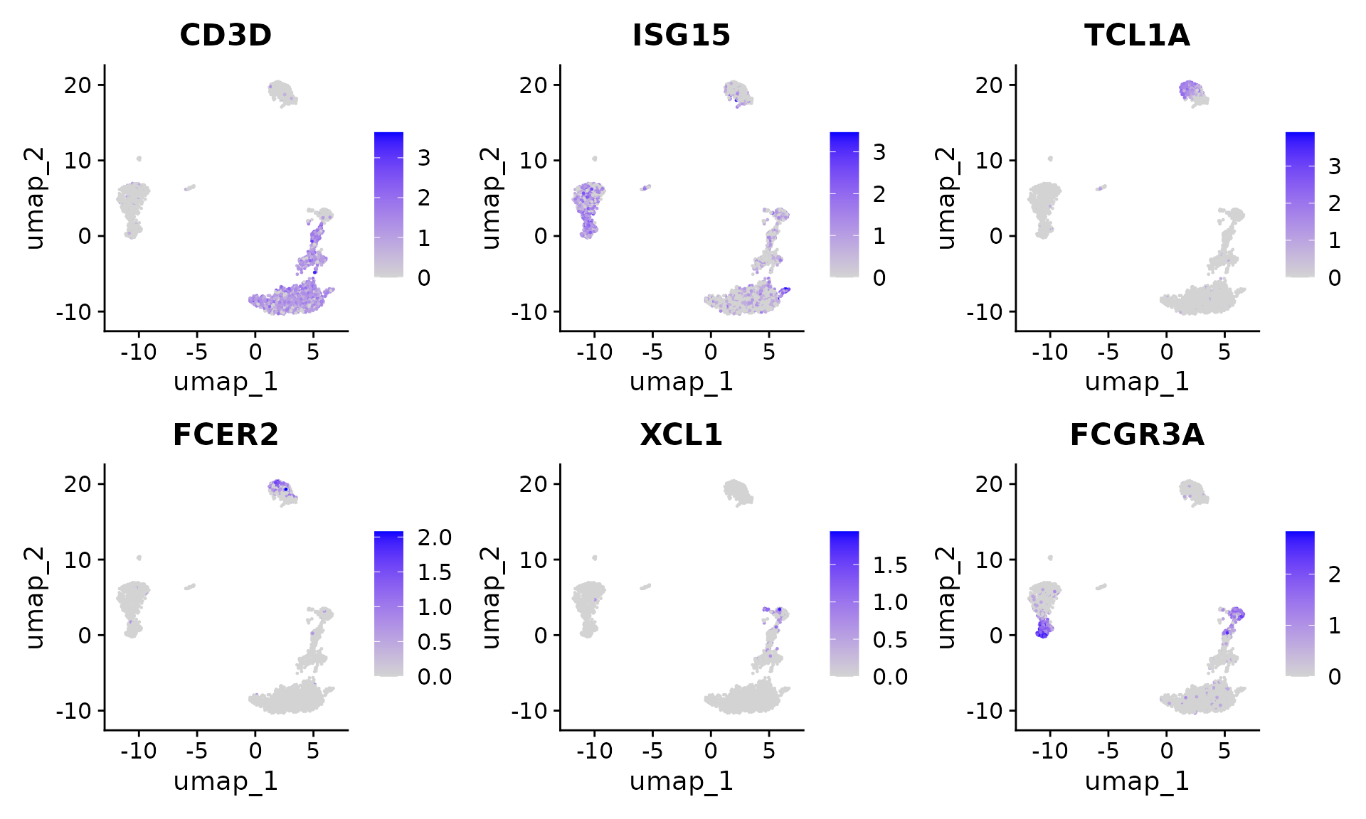
Session Info
## R version 4.5.2 (2025-10-31)
## Platform: x86_64-pc-linux-gnu
## Running under: Ubuntu 24.04.4 LTS
##
## Matrix products: default
## BLAS:   /usr/lib/x86_64-linux-gnu/openblas-pthread/libblas.so.3
## LAPACK: /usr/lib/x86_64-linux-gnu/openblas-pthread/libopenblasp-r0.3.26.so;  LAPACK version 3.12.0
##
## locale:
##  [1] LC_CTYPE=en_US.UTF-8       LC_NUMERIC=C
##  [3] LC_TIME=en_US.UTF-8        LC_COLLATE=en_US.UTF-8
##  [5] LC_MONETARY=en_US.UTF-8    LC_MESSAGES=en_US.UTF-8
##  [7] LC_PAPER=en_US.UTF-8       LC_NAME=C
##  [9] LC_ADDRESS=C               LC_TELEPHONE=C
## [11] LC_MEASUREMENT=en_US.UTF-8 LC_IDENTIFICATION=C
##
## time zone: Etc/UTC
## tzcode source: system (glibc)
##
## attached base packages:
## [1] stats     graphics  grDevices utils     datasets  methods   base
##
## other attached packages:
## [1] future_1.70.0      sctransform_0.4.3  ggplot2_4.0.3      Seurat_5.5.0
## [5] SeuratObject_5.4.0 sp_2.2-1
##
## loaded via a namespace (and not attached):
##   [1] RColorBrewer_1.1-3          jsonlite_2.0.0
##   [3] magrittr_2.0.5              ggbeeswarm_0.7.3
##   [5] spatstat.utils_3.2-2        farver_2.1.2
##   [7] rmarkdown_2.30              fs_2.1.0
##   [9] ragg_1.5.1                  vctrs_0.7.1
##  [11] ROCR_1.0-12                 DelayedMatrixStats_1.32.0
##  [13] spatstat.explore_3.8-0      S4Arrays_1.10.1
##  [15] htmltools_0.5.9             SparseArray_1.10.10
##  [17] sass_0.4.10                 parallelly_1.47.0
##  [19] KernSmooth_2.23-26          bslib_0.10.0
##  [21] htmlwidgets_1.6.4           desc_1.4.3
##  [23] ica_1.0-3                   plyr_1.8.9
##  [25] plotly_4.12.0               zoo_1.8-15
##  [27] cachem_1.1.0                igraph_2.3.0
##  [29] mime_0.13                   lifecycle_1.0.5
##  [31] pkgconfig_2.0.3             Matrix_1.7-5
##  [33] R6_2.6.1                    fastmap_1.2.0
##  [35] MatrixGenerics_1.22.0       fitdistrplus_1.2-6
##  [37] shiny_1.13.0                digest_0.6.39
##  [39] patchwork_1.3.2             S4Vectors_0.48.1
##  [41] tensor_1.5.1                RSpectra_0.16-2
##  [43] irlba_2.3.7                 GenomicRanges_1.62.1
##  [45] textshaping_1.0.5           beachmat_2.26.0
##  [47] labeling_0.4.3              progressr_0.19.0
##  [49] spatstat.sparse_3.1-0       httr_1.4.8
##  [51] polyclip_1.10-7             abind_1.4-8
##  [53] compiler_4.5.2              withr_3.0.2
##  [55] S7_0.2.1                    fastDummies_1.7.6
##  [57] R.utils_2.13.0              MASS_7.3-65
##  [59] DelayedArray_0.36.1         tools_4.5.2
##  [61] vipor_0.4.7                 lmtest_0.9-40
##  [63] otel_0.2.0                  beeswarm_0.4.0
##  [65] httpuv_1.6.16               future.apply_1.20.2
##  [67] goftest_1.2-3               R.oo_1.27.1
##  [69] glmGamPoi_1.22.0            glue_1.8.0
##  [71] nlme_3.1-168                promises_1.5.0
##  [73] grid_4.5.2                  Rtsne_0.17
##  [75] cluster_2.1.8.2             reshape2_1.4.5
##  [77] generics_0.1.4              gtable_0.3.6
##  [79] spatstat.data_3.1-9         R.methodsS3_1.8.2
##  [81] tidyr_1.3.2                 data.table_1.18.2.1
##  [83] XVector_0.50.0              BiocGenerics_0.56.0
##  [85] spatstat.geom_3.7-3         RcppAnnoy_0.0.23
##  [87] ggrepel_0.9.8               RANN_2.6.2
##  [89] pillar_1.11.1               stringr_1.6.0
##  [91] spam_2.11-3                 RcppHNSW_0.6.0
##  [93] later_1.4.8                 splines_4.5.2
##  [95] dplyr_1.2.0                 lattice_0.22-7
##  [97] survival_3.8-3              deldir_2.0-4
##  [99] tidyselect_1.2.1            miniUI_0.1.2
## [101] pbapply_1.7-4               knitr_1.51
## [103] gridExtra_2.3               Seqinfo_1.0.0
## [105] IRanges_2.44.0              SummarizedExperiment_1.40.0
## [107] scattermore_1.2             stats4_4.5.2
## [109] xfun_0.56                   Biobase_2.70.0
## [111] matrixStats_1.5.0           stringi_1.8.7
## [113] lazyeval_0.2.3              yaml_2.3.12
## [115] evaluate_1.0.5              codetools_0.2-20
## [117] tibble_3.3.1                cli_3.6.6
## [119] uwot_0.2.4                  xtable_1.8-8
## [121] reticulate_1.46.0           systemfonts_1.3.2
## [123] jquerylib_0.1.4             Rcpp_1.1.1-1.1
## [125] globals_0.19.1              spatstat.random_3.4-5
## [127] png_0.1-9                   ggrastr_1.0.2
## [129] spatstat.univar_3.1-7       parallel_4.5.2
## [131] pkgdown_2.2.0               dotCall64_1.2
## [133] sparseMatrixStats_1.22.0    listenv_0.10.1
## [135] viridisLite_0.4.3           scales_1.4.0
## [137] ggridges_0.5.7              purrr_1.2.1
## [139] rlang_1.2.0                 cowplot_1.2.0