Sketch integration using a 1 million cell dataset from Parse Biosciences
Compiled: 2026-05-12
Source:vignettes/ParseBio_sketch_integration.Rmd
ParseBio_sketch_integration.RmdThe recent increase in publicly available single-cell datasets poses a significant challenge for integrative analysis. For example, multiple tissues have now been profiled across dozens of studies, representing hundreds of individuals and millions of cells. In Hao et al, 2023 proposed a dictionary learning based method, atomic sketch integration, could also enable efficient and large-scale integrative analysis. Our procedure enables the integration of large compendiums of datasets without ever needing to load the full scale of data into memory. In our manuscript we use atomic sketch integration to integrate millions of scRNA-seq from human lung and human PBMC.
In this vignette, we demonstrate how to use atomic sketch integration to harmonize scRNA-seq experiments 1M cells, though we have used this procedure to integrate datasets of 10M+ cells as well. We analyze a dataset from Parse Biosciences, in which PBMC from 24 human samples (12 healthy donors, 12 Type-1 diabetes donors), which is available here.
- Sample a representative subset of cells (‘atoms’) from each dataset
- Integrate the atoms from each dataset, and define a set of cell states
- Reconstruct (integrate) the full datasets, based on the atoms
- Annotate all cells in the full datasets
- Identify cell-type specific differences between healthy and diabetic patients
Prior to running this vignette, please install Seurat v5, as well as the BPCells package, which we use for on-disk storage. You can read more about using BPCells in Seurat v5 here. We also recommend reading the Sketch-based analysis in Seurat v5 vignette, which introduces the concept of on-disk and in-memory storage in Seurat v5.
library(Seurat)
library(BPCells)
library(dplyr)
library(ggplot2)
library(ggrepel)
library(patchwork)
# set this option when analyzing large datasets
options(future.globals.maxSize = 5e+10)
Create a Seurat object containing data from 24 patients
We downloaded the original dataset and donor metadata from Parse
Biosciences. While the BPCells package can work directly with h5ad
files, for optimal performance, we converted the dataset to the
compressed sparse format used by BPCells, as described here. We create a
Seurat object for this dataset. Since the input to
CreateSeuratObject is a BPCells matrix, the data remains
on-disk and is not loaded into memory. After creating the object, we
split the dataset into 24 layers, one for each sample
(i.e. patient), to facilitate integration.
parse.mat <- open_matrix_dir(dir = "/brahms/hartmana/vignette_data/bpcells/parse_1m_pbmc")
# need to move
metadata <- readRDS("/brahms/haoy/vignette_data/ParseBio_PBMC_meta.rds")
object <- CreateSeuratObject(counts = parse.mat, meta.data = metadata)

object <- NormalizeData(object)
# split assay into 24 layers
object[["RNA"]] <- split(object[["RNA"]], f = object$sample)
object <- FindVariableFeatures(object, verbose = FALSE)
Sample representative cells from each dataset
Inspired by pioneering work aiming to identify ‘sketches’
of scRNA-seq data, our first step is to sample a representative set of
cells from each dataset. We compute a leverage score (estimate of ‘statistical leverage’) for
each cell, which helps to identify cells that are likely to be member of
rare subpopulations and ensure that these are included in our
representative sample. Importantly, the estimation of leverage scores
only requires data normalization, can be computed efficiently for sparse
datasets, and does not require any intensive computation or dimensional
reduction steps. We load each object separately, perform basic
preprocessing (normalization and variable feature selection), and select
and store 5,000 representative cells from each dataset. Since there are
24 datasets, the sketched dataset now contains 120,000 cells. These
cells are stored in a new sketch assay, and are loaded
in-memory.
object <- SketchData(object = object, ncells = 5000, method = "LeverageScore", sketched.assay = "sketch")
object
## An object of class Seurat
## 121328 features across 966344 samples within 2 assays
## Active assay: sketch (60664 features, 2000 variable features)
## 48 layers present: counts.H_3128, counts.H_3060, counts.H_409, counts.H_7108, counts.H_120, counts.D_504, counts.H_2928, counts.H_727, counts.H_4579, counts.H_6625, counts.H_630, counts.D_500, counts.D_501, counts.D_610, counts.H_4119, counts.D_609, counts.D_644, counts.D_498, counts.H_1334, counts.D_497, counts.D_505, counts.D_506, counts.D_502, counts.D_503, data.H_3128, data.H_3060, data.H_409, data.H_7108, data.H_120, data.D_504, data.H_2928, data.H_727, data.H_4579, data.H_6625, data.H_630, data.D_500, data.D_501, data.D_610, data.H_4119, data.D_609, data.D_644, data.D_498, data.H_1334, data.D_497, data.D_505, data.D_506, data.D_502, data.D_503
## 1 other assay present: RNAPerform integration on the sketched cells across samples
Next we perform integrative analysis on the ‘atoms’ from each of the
datasets. Here, we perform integration using the streamlined Seurat v5 integration workflow, and
utilize the reference-based RPCAIntegration method. The
function performs all corrections in low-dimensional space (rather than
on the expression values themselves) to further improve speed and memory
usage, and outputs a merged Seurat object where all cells have been
placed in an integrated low-dimensional space (stored as
integrated.rpca). However, we emphasize that you can
perform integration here using any analysis technique that places cells
across datasets into a shared space. This includes CCA Integration,
Harmony, and scVI. We demonstrate how to use these tools in Seurat v5 here.
DefaultAssay(object) <- "sketch"
object <- FindVariableFeatures(object, verbose = F)
object <- ScaleData(object, verbose = F)
object <- RunPCA(object, verbose = F)
# integrate the datasets
object <- IntegrateLayers(object, method = RPCAIntegration, orig = "pca", new.reduction = "integrated.rpca",
    dims = 1:30, k.anchor = 20, reference = which(Layers(object, search = "data") %in% c("data.H_3060")),
    verbose = F)
# cluster the integrated data
object <- FindNeighbors(object, reduction = "integrated.rpca", dims = 1:30)
object <- FindClusters(object, resolution = 2)
## Modularity Optimizer version 1.3.0 by Ludo Waltman and Nees Jan van Eck
##
## Number of nodes: 120000
## Number of edges: 5140371
##
## Running Louvain algorithm...
## Maximum modularity in 10 random starts: 0.8765
## Number of communities: 53
## Elapsed time: 102 seconds
object <- RunUMAP(object, reduction = "integrated.rpca", dims = 1:30, return.model = T, verbose = F)
# you can now rejoin the layers in the sketched assay this is required to perform differential
# expression
object[["sketch"]] <- JoinLayers(object[["sketch"]])
c10_markers <- FindMarkers(object = object, ident.1 = 10, max.cells.per.ident = 500, only.pos = TRUE)
head(c10_markers)
## p_val avg_log2FC pct.1 pct.2 p_val_adj
## NEAT1 1.390051e-90 1.681096 0.998 0.718 8.432605e-86
## SLC8A1 1.042114e-89 2.053690 0.916 0.275 6.321879e-85
## PID1 1.513628e-86 2.762468 0.839 0.174 9.182273e-82
## PSAP 2.538032e-79 2.040152 0.900 0.310 1.539672e-74
## LRP1 3.836166e-79 1.930123 0.821 0.228 2.327172e-74
## CYRIA 1.023813e-76 1.898088 0.901 0.347 6.210859e-72
# You can now annotate clusters using marker genes.  We performed this step, and include the
# results in the 'sketch.celltype' metadata column

plot.s1 <- DimPlot(object, group.by = "sample", reduction = "umap")
plot.s2 <- DimPlot(object, group.by = "celltype.manual", reduction = "umap")
plot.s1 + plot.s2 + plot_layout(ncol = 1)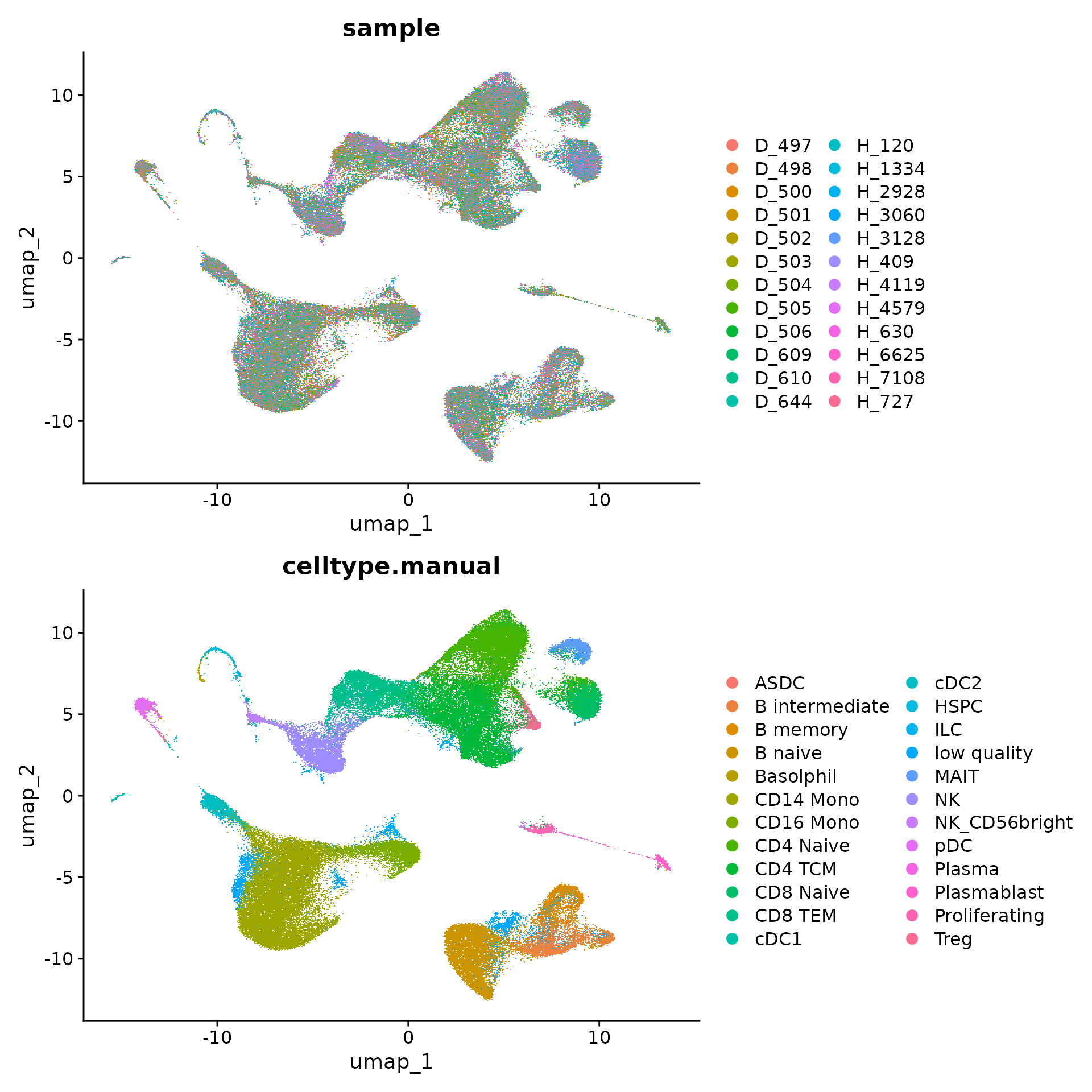
Integrate the full datasets
Now that we have integrated the subset of atoms of each dataset,
placing them each in an integrated low-dimensional space, we can now
place each cell from each dataset in this space as well. We load the
full datasets back in individually, and use the
ProjectIntegration function to integrate all cells. After
this function is run, the integrated.rpca.full space now
embeds all cells in the dataset.Even though all cells in the dataset
have been integrated together, the non-sketched cells are not loaded
into memory. Users can still switch between the sketch
(sketched cells, in-memory) and RNA (full dataset, on disk)
for analysis. After integration, we can also project cell type labels
from the sketched cells onto the full dataset using
ProjectData.
# resplit the sketched cell assay into layers this is required to project the integration onto
# all cells
object[["sketch"]] <- split(object[["sketch"]], f = object$sample)

object <- ProjectIntegration(object = object, sketched.assay = "sketch", assay = "RNA", reduction = "integrated.rpca")


object <- ProjectData(object = object, sketched.assay = "sketch", assay = "RNA", sketched.reduction = "integrated.rpca",
    full.reduction = "integrated.rpca.full", dims = 1:30, refdata = list(celltype.full = "celltype.manual"))
object <- RunUMAP(object, reduction = "integrated.rpca.full", dims = 1:30, reduction.name = "umap.full",
    reduction.key = "UMAP_full_")
p1 <- DimPlot(object, reduction = "umap.full", group.by = "sample", alpha = 0.1)
p2 <- DimPlot(object, reduction = "umap.full", group.by = "celltype.full", alpha = 0.1)

p1 + p2 + plot_layout(ncol = 1)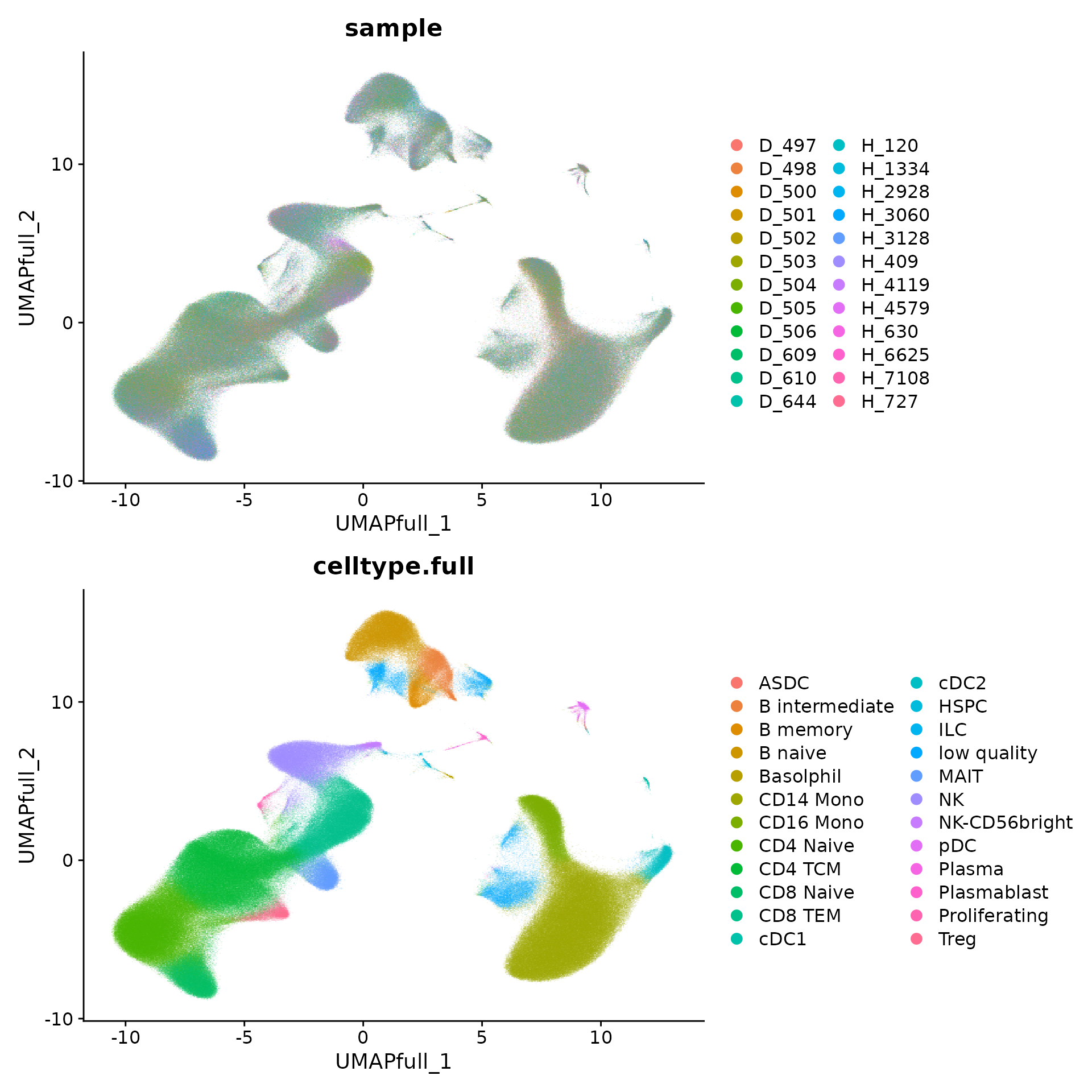
Compare healthy and diabetic samples
By integrating all samples together, we can now compare healthy and
diabetic cells in matched cell states. To maximize statistical power, we
want to use all cells - not just the sketched cells - to perform this
analysis. As recommended by Soneson et al. and
Crowell et
al., we use an aggregation-based (pseudobulk) workflow. We aggregate
all cells within the same cell type and sample using the
AggregateExpression function. This returns a Seurat object
where each ‘cell’ represents the pseudobulk profile of one cell type in
one individual.
After we aggregate cells, we can perform celltype-specific differential expression between healthy and diabetic samples using DESeq2. We demonstrate this for CD14 monocytes.
bulk <- AggregateExpression(object, return.seurat = T, slot = "counts", assays = "RNA", group.by = c("celltype.full",
"sample", "disease"))## [1] "Treg_H-4119_H" "Treg_H-4579_H" "Treg_H-630_H" "Treg_H-6625_H"
## [5] "Treg_H-7108_H" "Treg_H-727_H"
cd14.bulk <- subset(bulk, celltype.full == "CD14 Mono")
Idents(cd14.bulk) <- "disease"
de_markers <- FindMarkers(cd14.bulk, ident.1 = "D", ident.2 = "H", slot = "counts", test.use = "DESeq2",
    verbose = F)
de_markers$gene <- rownames(de_markers)
ggplot(de_markers, aes(avg_log2FC, -log10(p_val))) + geom_point(size = 0.5, alpha = 0.5) + theme_bw() +
    ylab("-log10(unadjusted p-value)") + geom_text_repel(aes(label = ifelse(p_val_adj < 0.01, gene,
    "")), colour = "red", size = 3)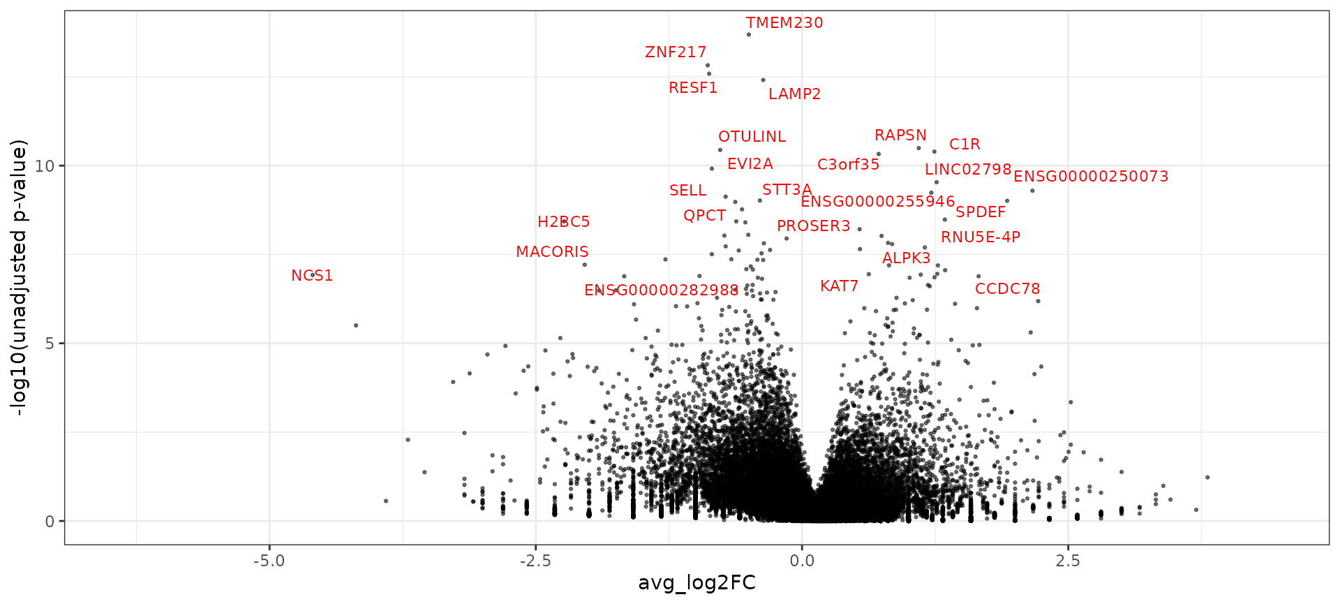
Session Info
## R version 4.5.2 (2025-10-31)
## Platform: x86_64-pc-linux-gnu
## Running under: Ubuntu 24.04.4 LTS
##
## Matrix products: default
## BLAS:   /usr/lib/x86_64-linux-gnu/openblas-pthread/libblas.so.3
## LAPACK: /usr/lib/x86_64-linux-gnu/openblas-pthread/libopenblasp-r0.3.26.so;  LAPACK version 3.12.0
##
## locale:
##  [1] LC_CTYPE=en_US.UTF-8       LC_NUMERIC=C
##  [3] LC_TIME=en_US.UTF-8        LC_COLLATE=en_US.UTF-8
##  [5] LC_MONETARY=en_US.UTF-8    LC_MESSAGES=en_US.UTF-8
##  [7] LC_PAPER=en_US.UTF-8       LC_NAME=C
##  [9] LC_ADDRESS=C               LC_TELEPHONE=C
## [11] LC_MEASUREMENT=en_US.UTF-8 LC_IDENTIFICATION=C
##
## time zone: Etc/UTC
## tzcode source: system (glibc)
##
## attached base packages:
## [1] stats     graphics  grDevices utils     datasets  methods   base
##
## other attached packages:
## [1] future_1.70.0      patchwork_1.3.2    ggrepel_0.9.8      ggplot2_4.0.3
## [5] dplyr_1.2.0        BPCells_0.3.1      Seurat_5.5.0       SeuratObject_5.4.0
## [9] sp_2.2-1
##
## loaded via a namespace (and not attached):
##   [1] RColorBrewer_1.1-3          jsonlite_2.0.0
##   [3] magrittr_2.0.5              spatstat.utils_3.2-2
##   [5] farver_2.1.2                rmarkdown_2.30
##   [7] fs_2.1.0                    ragg_1.5.1
##   [9] vctrs_0.7.1                 ROCR_1.0-12
##  [11] spatstat.explore_3.8-0      S4Arrays_1.10.1
##  [13] htmltools_0.5.9             SparseArray_1.10.10
##  [15] sass_0.4.10                 sctransform_0.4.3
##  [17] parallelly_1.47.0           KernSmooth_2.23-26
##  [19] bslib_0.10.0                htmlwidgets_1.6.4
##  [21] desc_1.4.3                  ica_1.0-3
##  [23] plyr_1.8.9                  plotly_4.12.0
##  [25] zoo_1.8-15                  cachem_1.1.0
##  [27] igraph_2.3.0                mime_0.13
##  [29] lifecycle_1.0.5             pkgconfig_2.0.3
##  [31] Matrix_1.7-5                R6_2.6.1
##  [33] fastmap_1.2.0               MatrixGenerics_1.22.0
##  [35] fitdistrplus_1.2-6          shiny_1.13.0
##  [37] digest_0.6.39               S4Vectors_0.48.1
##  [39] DESeq2_1.50.2               tensor_1.5.1
##  [41] RSpectra_0.16-2             irlba_2.3.7
##  [43] textshaping_1.0.5           GenomicRanges_1.62.1
##  [45] labeling_0.4.3              progressr_0.19.0
##  [47] spatstat.sparse_3.1-0       httr_1.4.8
##  [49] polyclip_1.10-7             abind_1.4-8
##  [51] compiler_4.5.2              withr_3.0.2
##  [53] S7_0.2.1                    BiocParallel_1.44.0
##  [55] fastDummies_1.7.6           MASS_7.3-65
##  [57] DelayedArray_0.36.1         tools_4.5.2
##  [59] lmtest_0.9-40               otel_0.2.0
##  [61] httpuv_1.6.16               future.apply_1.20.2
##  [63] goftest_1.2-3               glue_1.8.0
##  [65] nlme_3.1-168                promises_1.5.0
##  [67] grid_4.5.2                  Rtsne_0.17
##  [69] cluster_2.1.8.2             reshape2_1.4.5
##  [71] generics_0.1.4              gtable_0.3.6
##  [73] spatstat.data_3.1-9         tidyr_1.3.2
##  [75] data.table_1.18.2.1         XVector_0.50.0
##  [77] BiocGenerics_0.56.0         spatstat.geom_3.7-3
##  [79] RcppAnnoy_0.0.23            RANN_2.6.2
##  [81] pillar_1.11.1               stringr_1.6.0
##  [83] limma_3.66.0                spam_2.11-3
##  [85] RcppHNSW_0.6.0              later_1.4.8
##  [87] splines_4.5.2               lattice_0.22-7
##  [89] survival_3.8-3              deldir_2.0-4
##  [91] tidyselect_1.2.1            locfit_1.5-9.12
##  [93] miniUI_0.1.2                pbapply_1.7-4
##  [95] knitr_1.51                  gridExtra_2.3
##  [97] Seqinfo_1.0.0               IRanges_2.44.0
##  [99] SummarizedExperiment_1.40.0 scattermore_1.2
## [101] stats4_4.5.2                xfun_0.56
## [103] Biobase_2.70.0              statmod_1.5.1
## [105] matrixStats_1.5.0           stringi_1.8.7
## [107] lazyeval_0.2.3              yaml_2.3.12
## [109] evaluate_1.0.5              codetools_0.2-20
## [111] tibble_3.3.1                cli_3.6.6
## [113] uwot_0.2.4                  xtable_1.8-8
## [115] reticulate_1.46.0           systemfonts_1.3.2
## [117] jquerylib_0.1.4             Rcpp_1.1.1-1.1
## [119] globals_0.19.1              spatstat.random_3.4-5
## [121] png_0.1-9                   spatstat.univar_3.1-7
## [123] parallel_4.5.2              pkgdown_2.2.0
## [125] presto_1.0.0                dotCall64_1.2
## [127] listenv_0.10.1              viridisLite_0.4.3
## [129] scales_1.4.0                ggridges_0.5.7
## [131] purrr_1.2.1                 rlang_1.2.0
## [133] cowplot_1.2.0               formatR_1.14