Analysis, visualization, and integration of Visium HD spatial datasets with Seurat
Compiled: May 27, 2026
Source:vignettes/visiumhd_analysis_vignette.Rmd
visiumhd_analysis_vignette.RmdVisium HD support in Seurat
We have previously released support in Seurat for sequencing-based spatial transcriptomic (ST) technologies, including 10x Visium and SLIDE-seq. With Seurat v5.1+, we introduce support for analyzing data generated with Visium HD technology, which performs profiling at substantially higher spatial resolution than previous versions.
We note that Visium HD data is generated from spatially patterned oligonucleotides labeled in bins. However, since the data from this resolution is sparse, adjacent bins are pooled together to create and resolutions. 10x recommends the use of binned data for analysis, but Seurat supports in the simultaneous loading of multiple binnings, and will store them in a single object as different assays.
In this vignette, we provide an overview of some of the spatial workflows that Seurat supports for analyzing Visium HD data, in particular:
- Unsupervised clustering
- Identification of spatial tissue domains
- Subsetting spatial regions
- Integration with scRNA-seq data
- Comparing the spatial localization of different cell types
We strongly encourage users to explore how different parameter settings affect their results, to analyze data iteratively (and in collaboration with biological experts), and to orthogonally validate unexpected or surprising biological findings.
In this vignette, we focus our analysis on a Visium HD dataset from the mouse brain, but also run the clustering workflow on a Visium HD dataset from the mouse small intestine. Links to access and download these data from the 10x repository are available in their respective sections.
First, we load Seurat and the other packages necessary for this vignette. Core functionality in support of Visium HD data was initially introduced in Seurat v5.1.0.
# packages required for Visium HD
install.packages("hdf5r")
install.packages("arrow")Load Visium HD data
The Visium HD mouse brain dataset is available for download here.
Seurat can load and store multiple binnings/resolutions in different
assays–the bin.size parameter specifies which resolutions
to load, with
and
bins loaded by default. For analysis, users can switch between
resolutions by changing
the default assay.
localdir <- "/brahms/shared/vignette-data/visium_hd_mouse_brain"
object <- Load10X_Spatial(data.dir = localdir, bin.size = c(8, 16))
# Setting the default assay changes analysis target between 8um and 16um binning
Assays(object)
## [1] "Spatial.008um" "Spatial.016um"
DefaultAssay(object) <- "Spatial.008um"
vln.plot <- VlnPlot(object, features = 'nCount_Spatial.008um', pt.size = 0) +
              theme(axis.text = element_text(size = 4)) + NoLegend()

count.plot <- SpatialFeaturePlot(object, features = 'nCount_Spatial.008um') +
                theme(legend.position = "right")

# Note that many spots have very few counts, in-part due to low cellular density in certain tissue regions
vln.plot | count.plot
Normalize datasets
In this vignette, we use standard log-normalization for spatial data. We note that the best normalization methods for spatial data are still being developed and evaluated, and encourage users to read manuscripts from the Phipson/Davis and Fan labs to learn more about potential caveats for spatial normalization.
# Normalize both 8um and 16um bins
DefaultAssay(object) <- "Spatial.008um"
object <- NormalizeData(object)

DefaultAssay(object) <- "Spatial.016um"
object <- NormalizeData(object)
Visualize gene expression
In this section, we visualize the expression of selected genes in the
Visium HD dataset. This allows us to observe spatial patterns of gene
expression and correlate them with histological features. We encourage
users to explore the different parameters available for
adjustment–including pt.size.factor, shape,
and stroke, among others–through function
documentation.
# Switch spatial resolution to 16um from 8um
DefaultAssay(object) <- "Spatial.016um"
p1 <- SpatialFeaturePlot(object, features = "Rorb") + ggtitle("Rorb expression (16um)")

# Switch back to 8um
DefaultAssay(object) <- "Spatial.008um"
p2 <- SpatialFeaturePlot(object, features = "Hpca") + ggtitle("Hpca expression (8um)")

p1 | p2
Unsupervised clustering
While the standard scRNA-seq clustering workflow can also be applied to spatial datasets, we have observed that when working with Visium HD datasets, the Seurat v5 sketch clustering workflow exhibits improved performance, especially for identifying rare and spatially restricted groups.
As described in Hao et al, 2023 and Hie et al, 2019, sketch-based analyses aim to ‘subsample’ large datasets in a way that preserves rare populations. Here, we sketch the Visium HD dataset, perform clustering on the subsampled cells, and then project the cluster labels back to the full dataset.
Details of the sketching procedure and workflow are described in Hao et al, 2023 and the Seurat v5 sketch-based analysis vignette. Since the full Visium HD dataset fits in memory, we do not use any of the on-disk capabilities of Seurat v5 in this vignette.
# Note that data is already normalized
DefaultAssay(object) <- "Spatial.008um"
object <- FindVariableFeatures(object)
object <- ScaleData(object)

# We select 50,0000 cells and create a new 'sketch' assay
object <- SketchData(object = object,
                     ncells = 50000,
                     method = "LeverageScore",
                     sketched.assay = "sketch")
# Switch analysis to sketched cells
DefaultAssay(object) <- "sketch"

# Perform the clustering workflow
object <- FindVariableFeatures(object)
object <- ScaleData(object)
object <- RunPCA(object, assay = "sketch", reduction.name = "pca.sketch")
object <- FindNeighbors(object, assay = "sketch", reduction = "pca.sketch", dims = 1:50)
object <- FindClusters(object, cluster.name = "seurat_cluster.sketched", resolution = 3)
## Modularity Optimizer version 1.3.0 by Ludo Waltman and Nees Jan van Eck
##
## Number of nodes: 50000
## Number of edges: 2098963
##
## Running Louvain algorithm...
## Maximum modularity in 10 random starts: 0.7811
## Number of communities: 61
## Elapsed time: 27 seconds
object <- RunUMAP(object, reduction = "pca.sketch", reduction.name = "umap.sketch", return.model = T, dims = 1:50)Now we can project the cluster labels and dimensional reductions (PCA
and UMAP), which we learned from the 50,000 sketched cells, to the
entire dataset using the ProjectData function.
In the resulting object, for all cells:
- Cluster labels are stored in
object$seurat_cluster.projected - Projected PCA embeddings are stored in
object[["pca.008um"]] - Projected UMAP embeddings are stored in
object[["umap.sketch"]]
object <- ProjectData(
  object = object,
  assay = "Spatial.008um",
  full.reduction = "full.pca.sketch",
  sketched.assay = "sketch",
  sketched.reduction = "pca.sketch",
  umap.model = "umap.sketch",
  dims = 1:50,
  refdata = list(seurat_cluster.projected = "seurat_cluster.sketched")
)
We can visualize the clustering results for the sketched cells, as well as the projected clustering results for the full dataset:
DefaultAssay(object) <- "sketch"
Idents(object) <- "seurat_cluster.sketched"
p1 <- DimPlot(object, reduction = "umap.sketch", label=F) + ggtitle("Sketched clustering (50,000 cells)") + theme(legend.position = "bottom")

# switch to full dataset
DefaultAssay(object) <- "Spatial.008um"
Idents(object) <- "seurat_cluster.projected"
p2 <- DimPlot(object, reduction = "full.umap.sketch", label=F) + ggtitle("Projected clustering (full dataset)") + theme(legend.position = "bottom")

p1 | p2
Of course, we can now also visualize the unsupervised clusters based
on their spatial location. Note that running
SpatialDimPlot(object, interactive = TRUE), also enables
interactive visualization and exploration.
SpatialDimPlot(object, label = T, repel = T, label.size = 4)
When there are many different clusters (some of which are spatially restricted and others are mixed), plotting the spatial location of all clusters can be challenging to interpret. We find it helpful to plot the spatial location of different clusters individually. For example, we highlight the spatial localization of a few clusters below, which happen to correspond to different cortical layers:
Idents(object) <- "seurat_cluster.projected"
cells <- CellsByIdentities(object, idents=c(0,4,30,34,35))
p <- SpatialDimPlot(object, cells.highlight = cells[setdiff(names(cells), "NA")],
                    cols.highlight = c("#FFFF00","grey50"), facet.highlight = T, combine=T) + NoLegend()
p
We can also find and visualize the top gene expression markers for each cluster:
# Crete downsampled object to make visualization either
DefaultAssay(object) <- "Spatial.008um"
Idents(object) <- "seurat_cluster.projected"
object_subset <- subset(object, cells = Cells(object[['Spatial.008um']]), downsample=1000)

# Order clusters by similarity
DefaultAssay(object_subset) <- "Spatial.008um"
Idents(object_subset) <- "seurat_cluster.projected"
object_subset <- BuildClusterTree(object_subset, assay = "Spatial.008um", reduction = "full.pca.sketch", reorder = T)

markers <- FindAllMarkers(object_subset, assay = 'Spatial.008um', only.pos = TRUE)
markers %>%
  group_by(cluster) %>%
  dplyr::filter(avg_log2FC > 1) %>%
  slice_head(n = 5) %>%
  ungroup() -> top5

object_subset <- ScaleData(object_subset, assay = "Spatial.008um", features = top5$gene)
p <- DoHeatmap(object_subset, assay = "Spatial.008um", features = top5$gene, size = 2.5) + theme(axis.text = element_text(size = 5.5)) + NoLegend()
p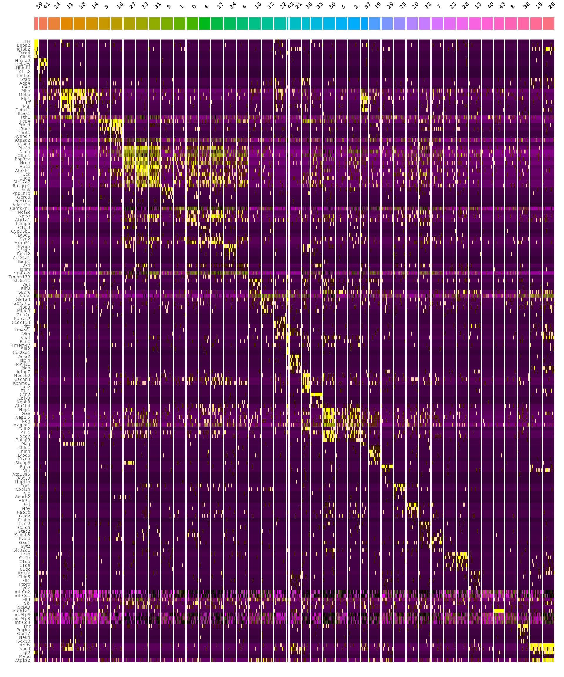
Identifying spatially-defined tissue domains
While the previous analyses consider each bin independently, spatial data enables cells to be defined not just by their neighborhood, but also by their broader spatial context.
In Singhal et al., the authors introduce BANKSY, Building Aggregates with a Neighborhood Kernel and Spatial Yardstick (BANKSY). BANKSY performs multiple tasks, but we find it particularly valuable for identifying and segmenting tissue domains. When performing clustering, BANKSY augments a spot’s expression pattern with both the mean and the gradient of gene expression levels in a spot’s broader neighborhood.
We thank the authors for enabling BANKSY to be compatible with Seurat
via the SeuratWrappers
framework, which requires separate installation of the BANKSY
package:
if (!requireNamespace("Banksy", quietly = TRUE)) {
  remotes::install_github("prabhakarlab/Banksy@devel")
}
library(SeuratWrappers)
library(Banksy)
Before running BANKSY, there are two important model parameters that users should consider:
-
k_geom: Local neighborhood size. Larger values will yield larger domains -
lambda: Influence of the neighborhood. Larger values yield more spatially coherent domains
The RunBanksy function creates a new BANKSY
assay, which can be used for dimensional reduction and clustering:
object <- RunBanksy(object, lambda = 0.8, verbose=TRUE,
                    assay = 'Spatial.008um', slot = 'data', features = 'variable',
                    k_geom = 50)
DefaultAssay(object) <- "BANKSY"
object <- RunPCA(object, assay = 'BANKSY', reduction.name = "pca.banksy", features = rownames(object), npcs = 30)
object <- FindNeighbors(object, reduction = "pca.banksy", dims = 1:30)
object <- FindClusters(object, cluster.name = "banksy_cluster", resolution = 0.5)
## Modularity Optimizer version 1.3.0 by Ludo Waltman and Nees Jan van Eck
##
## Number of nodes: 393543
## Number of edges: 9956157
##
## Running Louvain algorithm...
## Maximum modularity in 10 random starts: 0.9469
## Number of communities: 30
## Elapsed time: 201 seconds
Idents(object) <- "banksy_cluster"
p <- SpatialDimPlot(object, images = "slice1.008um", group.by = "banksy_cluster", label = T, repel = T, label.size = 4)
p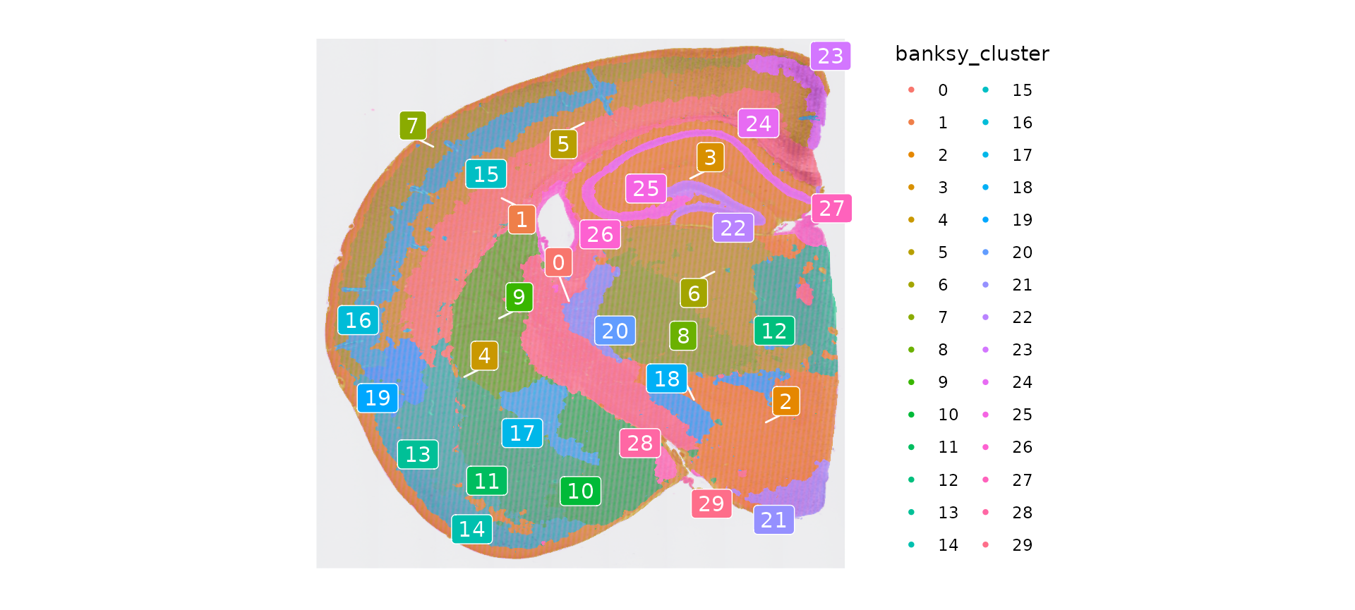
As with unsupervised clustering, we can highlight the spatial location of each tissue domain individually:
banksy_cells <- CellsByIdentities(object)
p <- SpatialDimPlot(object, cells.highlight = banksy_cells[setdiff(names(banksy_cells), "NA")], cols.highlight = c("#FFFF00","grey50"),facet.highlight = T, combine=T) + NoLegend()
p
Subset out anatomical regions
Users may wish to segment or subset out a restricted region for
further downstream analysis. For example, here we create a
coordinate-defined segmentation mask marking cortical and hippocampal
regions from the entire dataset using the
CreateSegmentation function, and then identify cells that
fall into this region with the Overlay function.
The list of coordinates is available for download here,
and users can identify these boundaries when exploring their own
datasets using the interactive=TRUE argument to
SpatialDimPlot.
cortex.coordinates <- as.data.frame(read.csv('/brahms/lis/visium_hd/final_mouse/cortex-hippocampus_coordinates.csv'))
cortex <- CreateSegmentation(cortex.coordinates)

object[["cortex"]] <- Overlay(object[["slice1.008um"]], cortex)
cortex <- subset(object, cells=Cells(object[['cortex']]))
Integration with scRNA-seq data (deconvolution)
Seurat v5 also includes support for Robust Cell Type Decomposition, a computational approach to deconvolve spot-level data from spatial datasets, when provided with an scRNA-seq reference. RCTD has been shown to accurately annotate spatial data from a variety of technologies, including SLIDE-seq, Visium, and the 10x Xenium in-situ spatial platform. We observe good performance with Visium HD as well.
To run RCTD, we first install the spacexr package from
GitHub which implements RCTD. When running RCTD, we follow the
instructions from the RCTD
vignette.
if (!requireNamespace("spacexr", quietly = TRUE)) {
  devtools::install_github("dmcable/spacexr", build_vignettes = FALSE)
}
library(spacexr)
RCTD takes an scRNA-seq dataset as a reference, and a spatial dataset as a query. For a reference, we use a mouse scRNA-seq dataset from the Allen Brain Atlas, available for download here. The reference scRNAs-eq dataset has been reduced to 200,000 cells (and rare cell types <25 cells have been removed).
We use the cortex Visium HD object as the spatial query. For computational efficiency, we sketch the spatial query dataset, apply RCTD to deconvolute the ‘sketched’ cortical cells and annotate them, and then project these annotations to the full cortical dataset.
#sketch the cortical subset of the Visium HD dataset
DefaultAssay(cortex) <- "Spatial.008um"
cortex <- FindVariableFeatures(cortex)
cortex <- SketchData(
  object = cortex,
  ncells = 50000,
  method = "LeverageScore",
  sketched.assay = "sketch"
)

DefaultAssay(cortex) <- "sketch"
cortex <- ScaleData(cortex)
cortex <- RunPCA(cortex, assay="sketch", reduction.name = "pca.cortex.sketch", verbose = T)
cortex <- FindNeighbors(cortex, reduction = "pca.cortex.sketch", dims = 1:50)
cortex <- RunUMAP(cortex, reduction = "pca.cortex.sketch", reduction.name = "umap.cortex.sketch", return.model = T, dims = 1:50, verbose = T)
# load in the reference scRNA-seq dataset
ref <- readRDS("/brahms/satijar/allen_scRNAseq_ref.Rds")
Idents(ref) <- "subclass_label"
counts <- ref[["RNA"]]$counts
cluster <- as.factor(ref$subclass_label)
nUMI <- ref$nCount_RNA
levels(cluster) <- gsub("/", "-", levels(cluster))
cluster <- droplevels(cluster)

# create the RCTD reference object
reference <- Reference(counts, cluster, nUMI)

counts_hd <- cortex[["sketch"]]$counts
cortex_cells_hd <- colnames(cortex[["sketch"]])
coords <- GetTissueCoordinates(cortex)[cortex_cells_hd,1:2]

# create the RCTD query object
query <- SpatialRNA(coords, counts_hd, colSums(counts_hd))
# run RCTD
RCTD <- create.RCTD(query, reference, max_cores = 28)
RCTD <- run.RCTD(RCTD, doublet_mode = "doublet")
# add results back to Seurat object
cortex <- AddMetaData(cortex, metadata = RCTD@results$results_df)
# project RCTD labels from sketched cortical cells to all cortical cells
cortex$first_type <- as.character(cortex$first_type)
cortex$first_type[is.na(cortex$first_type)] <- 'Unknown'
cortex <- ProjectData(
  object = cortex,
  assay = "Spatial.008um",
  full.reduction = "pca.cortex",
  sketched.assay = "sketch",
  sketched.reduction = "pca.cortex.sketch",
  umap.model = "umap.cortex.sketch",
  dims = 1:50,
  refdata = list(full_first_type = "first_type")
)
DefaultAssay(object) <- "Spatial.008um"

# we only ran RCTD on the cortical cells
# set labels to all other cells as "Unknown"
object[[]][, "full_first_type"] <- "Unknown"
object$full_first_type[Cells(cortex)] <- cortex$full_first_type[Cells(cortex)]
Idents(object) <- 'full_first_type'

# now we can spatially map the location of any scRNA-seq cell type
# start with Layered (starts with L), excitatory neurons in the cortex
cells <- CellsByIdentities(object)
excitatory_names <- sort(grep("^L.* CTX",names(cells),value = TRUE))
p <- SpatialDimPlot(object, cells.highlight = cells[excitatory_names], cols.highlight = c("#FFFF00","grey50"), facet.highlight = T, combine=T, ncol=4)
p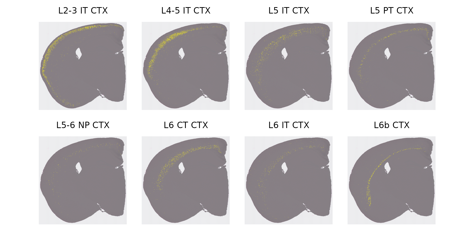
We can now look for associations between the scRNA-seq labels of individual bins, and their tissue domain identity (as assigned by BANKSY). By asking which domains the excitatory neuron cells fall in, we can rename the BANKSY clusters as neuronal layers:
plot_cell_types <- function(data, label) {
  p <- ggplot(data, aes(x = get(label), y = n, fill = full_first_type)) +
    geom_bar(stat = "identity", position = "stack") +
    geom_text(aes(label = ifelse(n >= min_count_to_show_label, full_first_type, "")), position = position_stack(vjust = 0.5), size = 2) +
    xlab(label) +
    ylab("# of Spots") +
    ggtitle(paste0("Distribution of Cell Types across ", label)) +
    theme_minimal()
}

cell_type_banksy_counts <- object[[]] %>%
  dplyr::filter(full_first_type %in% excitatory_names) %>%
  dplyr::count(full_first_type, banksy_cluster)

min_count_to_show_label <- 20

p <- plot_cell_types(cell_type_banksy_counts, "banksy_cluster")
p
Based on this plot, we can now assign cells (even if they are not excitatory neurons) to individual neuronal layers.
Idents(object) <- 'banksy_cluster'
object$layer_id <- 'Unknown'
object$layer_id[WhichCells(object,idents = c(5))] <- "Layer 2/3"
object$layer_id[WhichCells(object,idents = c(12))] <- "Layer 4"
object$layer_id[WhichCells(object,idents = c(7))] <- "Layer 5"
object$layer_id[WhichCells(object,idents = c(3))] <- "Layer 6"
Finally, we can visualize the spatial distribution of other cell types, and ask which cortical layers they fall in. For example, in contrast to excitatory neurons, inhibitory (GABAergic) interneurons in the cortex are not spatially restricted to individual layers - but they do show biases.
In our previous analysis of STARmap data, and consistent with previous work, we found that SST and PV interneuron classes tend to be restricted to layers 4-6, while VIP and Lamp5 interneurons tend to be located in layers 2/3. These results were based on an in-situ imaging technology which captures single-cell profiles - and here we ask whether we can find the same result in Visium HD spot-based data.
# set ID to RCTD label
Idents(object) <- 'full_first_type'

# Visualize distribution of 4 interneuron subtypes
inhibitory_names <- c("Sst","Pvalb","Vip","Lamp5")
cell_ids <- CellsByIdentities(object, idents = inhibitory_names)
p <- SpatialDimPlot(object, cells.highlight = cell_ids, cols.highlight = c("#FFFF00","grey50"), facet.highlight = T, combine=T, ncol=4)
p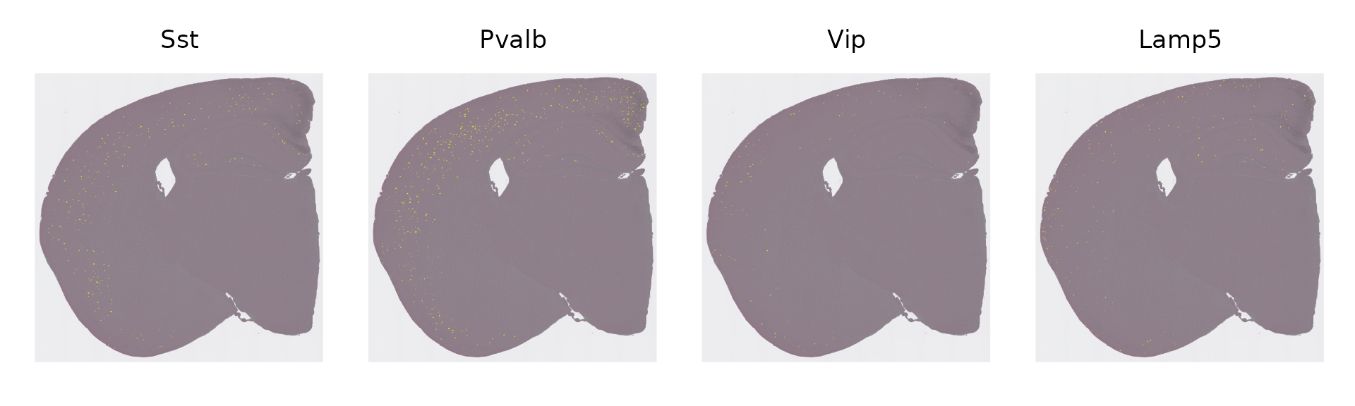
# create barplot to show proportions of cell types of interest
layer_table <- table(object$full_first_type, object$layer_id)[inhibitory_names,1:4]

neuron_props <- reshape2::melt(prop.table(layer_table), margin = 1)
ggplot(neuron_props, aes(x = Var1, y = value, fill = Var2)) +
  geom_bar(stat = "identity", position = "fill") +
  labs(x = "Cell type", y = "Proportion", fill = "Layer") +
  theme_classic()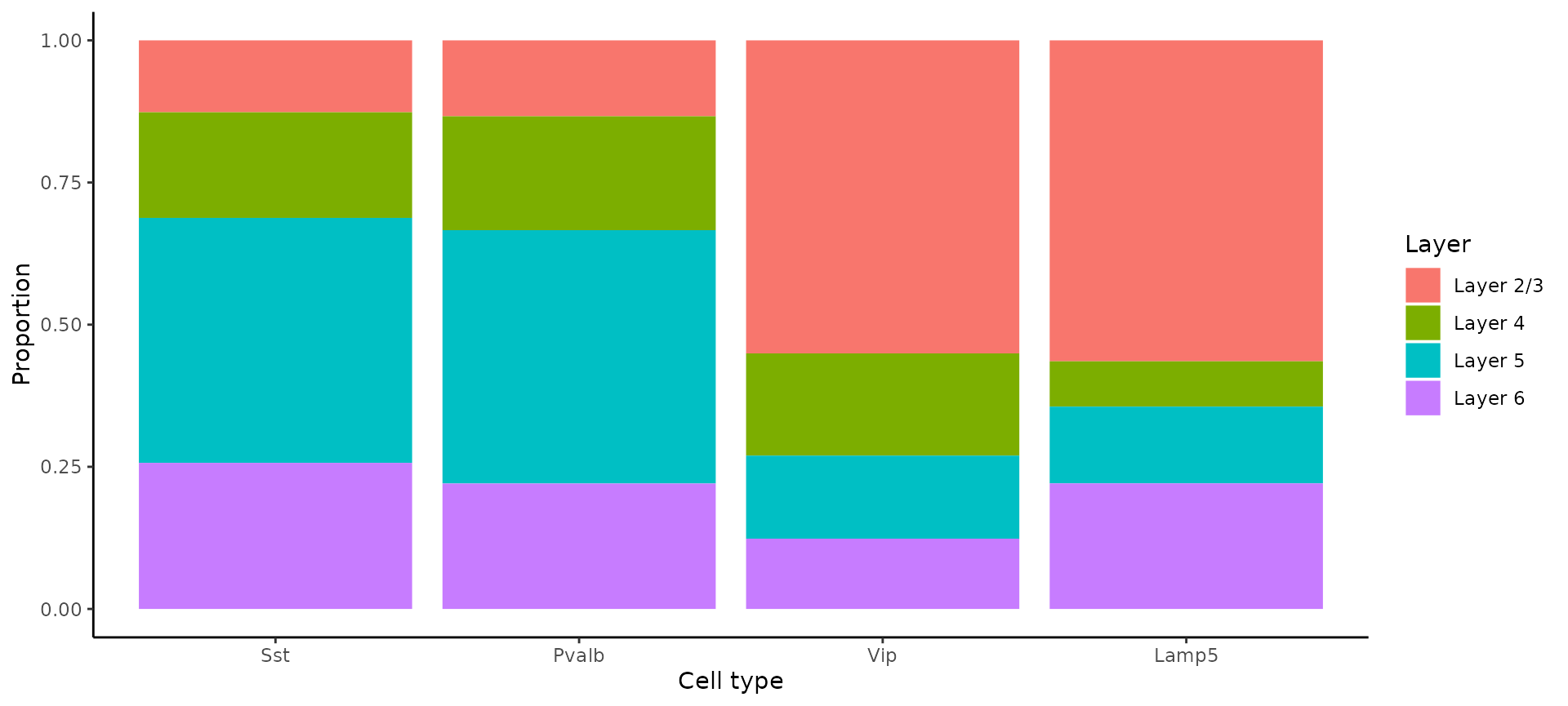
We recapitulate the same findings, previously identified in in-situ imaging data, in the Visium HD dataset. This highlights that the 8um binning of Visium HD, even though it does not represent true single cell resolution, is capable of accurately localizing scRNA-seq-defined cell types, although we strongly encourage users to orthogonally validate unexpected or surprising biological findings.
Unsupervised clustering: mouse intestine
We briefly demonstrate our sketch-clustering workflow on a second Visium HD dataset, from the Mouse Small Intestine (FFPE), available for download here. We identify clusters, visualize their spatial locations, and report their top gene expression markers:
localdir <- "/brahms/lis/visium_hd/Visium_HD_Public_Data/HD_public_data/Visium_HD_Mouse_Small_Intestine/outs"
object <- Load10X_Spatial(data.dir = localdir, bin.size = 8)
DefaultAssay(object) <- "Spatial.008um"
object <- NormalizeData(object)
object <- FindVariableFeatures(object)
object <- ScaleData(object)
object <- SketchData(
  object = object,
  ncells = 50000,
  method = "LeverageScore",
  sketched.assay = "sketch"
)
DefaultAssay(object) <- "sketch"
object <- FindVariableFeatures(object)
object <- ScaleData(object)
object <- RunPCA(object, assay="sketch", reduction.name = "pca.sketch")
object <- FindNeighbors(object, assay="sketch", reduction = "pca.sketch", dims = 1:50)
object <- FindClusters(object, cluster.name="seurat_cluster.sketched", resolution = 3)
## Modularity Optimizer version 1.3.0 by Ludo Waltman and Nees Jan van Eck
##
## Number of nodes: 50000
## Number of edges: 2104989
##
## Running Louvain algorithm...
## Maximum modularity in 10 random starts: 0.7670
## Number of communities: 45
## Elapsed time: 25 seconds
object <- RunUMAP(object, reduction = "pca.sketch", reduction.name = "umap.sketch", return.model = T, dims = 1:50)
object <- ProjectData(
  object = object,
  assay = "Spatial.008um",
  full.reduction = "full.pca.sketch",
  sketched.assay = "sketch",
  sketched.reduction = "pca.sketch",
  umap.model = "umap.sketch",
  dims = 1:50,
  refdata = list(seurat_cluster.projected = "seurat_cluster.sketched")
)
Idents(object) <- "seurat_cluster.projected"
DefaultAssay(object) <- "Spatial.008um"

p1 <- DimPlot(object, reduction = "umap.sketch", label=F) + theme(legend.position = "bottom")
p2 <- SpatialDimPlot(object, label=F) + theme(legend.position = "bottom")
p1 | p2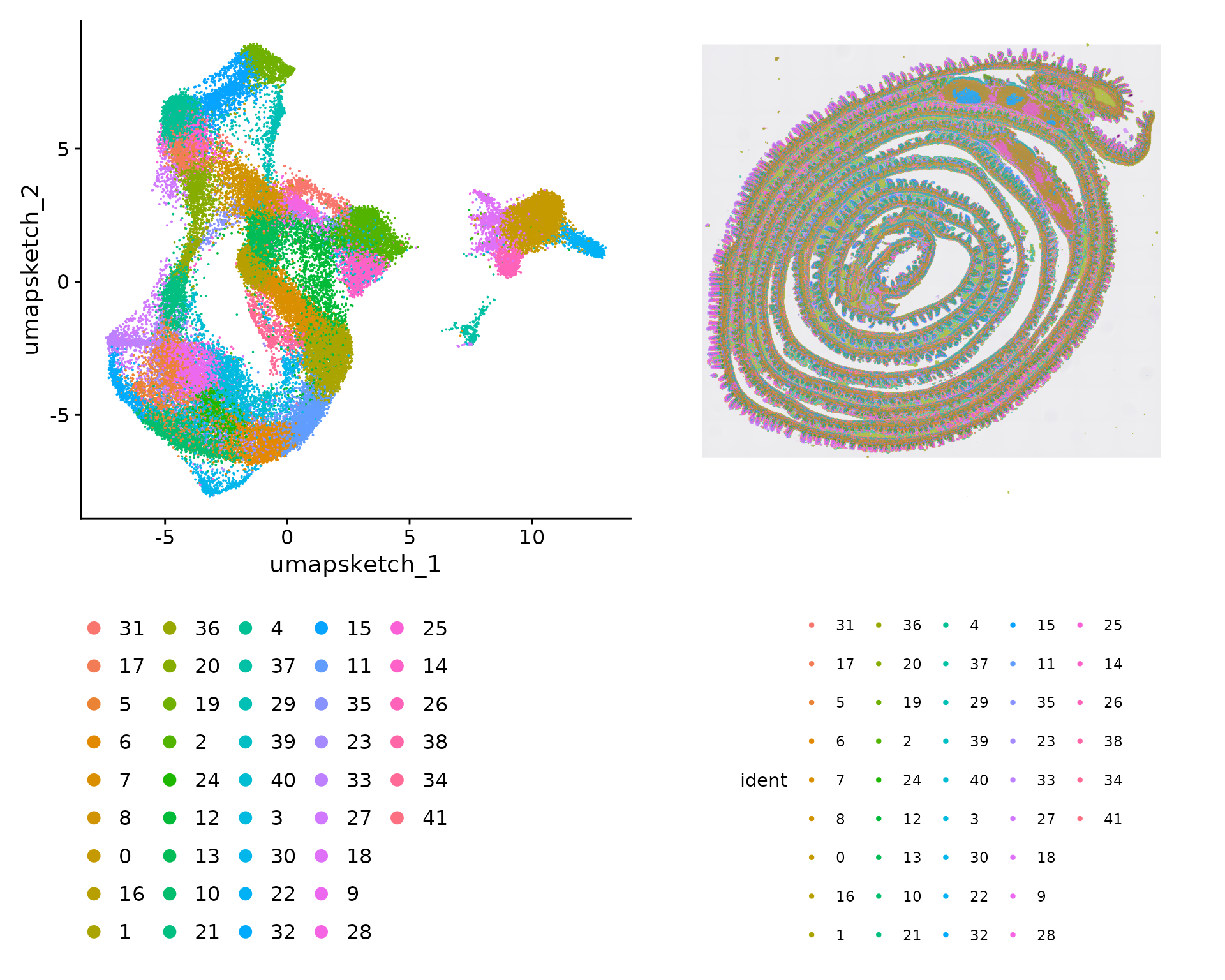
We visualize the location of each cluster individually:
Idents(object) <- "seurat_cluster.projected"
cells <- CellsByIdentities(object, idents=c(1,5,18,26))
p <- SpatialDimPlot(object, cells.highlight = cells[setdiff(names(cells), "NA")], cols.highlight = c("#FFFF00","grey50"), facet.highlight = T, combine=T) + NoLegend()
p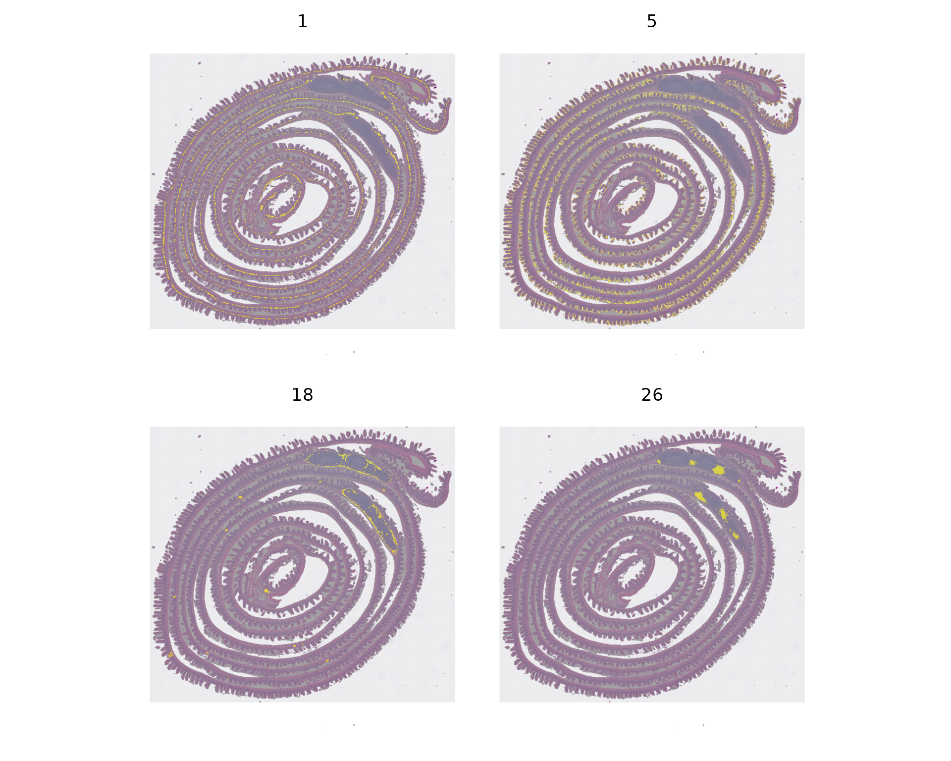
DefaultAssay(object) <- "Spatial.008um"
Idents(object) <- "seurat_cluster.projected"
object_subset <- subset(object, cells = Cells(object[['Spatial.008um']]), downsample=1000)

DefaultAssay(object_subset) <- "Spatial.008um"
Idents(object_subset) <- "seurat_cluster.projected"
object_subset <- BuildClusterTree(object_subset, assay = "Spatial.008um", reduction = "full.pca.sketch", reorder = T)

markers <- FindAllMarkers(object_subset, assay = "Spatial.008um", only.pos = TRUE)
markers %>%
  group_by(cluster) %>%
  dplyr::filter(avg_log2FC > 1) %>%
  slice_head(n = 5) %>%
  ungroup() -> top5

object_subset <- ScaleData(object_subset, assay = "Spatial.008um", features=top5$gene)
p <- DoHeatmap(object_subset, assay = "Spatial.008um", features = top5$gene, size = 2.5) + theme(axis.text = element_text(size = 5.5)) + NoLegend()
p
Session Info
## R version 4.5.2 (2025-10-31)
## Platform: x86_64-pc-linux-gnu
## Running under: Ubuntu 24.04.4 LTS
##
## Matrix products: default
## BLAS:   /usr/lib/x86_64-linux-gnu/openblas-pthread/libblas.so.3
## LAPACK: /usr/lib/x86_64-linux-gnu/openblas-pthread/libopenblasp-r0.3.26.so;  LAPACK version 3.12.0
##
## locale:
##  [1] LC_CTYPE=en_US.UTF-8       LC_NUMERIC=C
##  [3] LC_TIME=en_US.UTF-8        LC_COLLATE=en_US.UTF-8
##  [5] LC_MONETARY=en_US.UTF-8    LC_MESSAGES=en_US.UTF-8
##  [7] LC_PAPER=en_US.UTF-8       LC_NAME=C
##  [9] LC_ADDRESS=C               LC_TELEPHONE=C
## [11] LC_MEASUREMENT=en_US.UTF-8 LC_IDENTIFICATION=C
##
## time zone: Etc/UTC
## tzcode source: system (glibc)
##
## attached base packages:
## [1] stats     graphics  grDevices utils     datasets  methods   base
##
## other attached packages:
##  [1] spacexr_2.2.1        Banksy_1.9.1         SeuratWrappers_0.4.0
##  [4] future_1.70.0        dplyr_1.2.1          patchwork_1.3.2
##  [7] ggplot2_4.0.3        Seurat_5.5.0         SeuratObject_5.4.0
## [10] sp_2.2-1
##
## loaded via a namespace (and not attached):
##   [1] RcppHungarian_0.3           RcppAnnoy_0.0.23
##   [3] splines_4.5.2               later_1.4.8
##   [5] R.oo_1.27.1                 tibble_3.3.1
##   [7] polyclip_1.10-7             fastDummies_1.7.6
##   [9] lifecycle_1.0.5             sf_1.1-0
##  [11] aricode_1.0.3               doParallel_1.0.17
##  [13] globals_0.19.1              lattice_0.22-7
##  [15] hdf5r_1.3.12                MASS_7.3-65
##  [17] magrittr_2.0.5              limma_3.66.0
##  [19] plotly_4.12.0               sass_0.4.10
##  [21] rmarkdown_2.31              remotes_2.5.0
##  [23] jquerylib_0.1.4             yaml_2.3.12
##  [25] httpuv_1.6.16               otel_0.2.0
##  [27] sctransform_0.4.3           spam_2.11-3
##  [29] spatstat.sparse_3.1-0       reticulate_1.46.0
##  [31] DBI_1.3.0                   cowplot_1.2.0
##  [33] pbapply_1.7-4               RColorBrewer_1.1-3
##  [35] abind_1.4-8                 quadprog_1.5-8
##  [37] Rtsne_0.17                  GenomicRanges_1.62.1
##  [39] R.utils_2.13.0              purrr_1.2.1
##  [41] presto_1.0.0                BiocGenerics_0.56.0
##  [43] IRanges_2.44.0              S4Vectors_0.48.1
##  [45] ggrepel_0.9.8               irlba_2.3.7
##  [47] listenv_0.10.1              spatstat.utils_3.2-2
##  [49] units_1.0-1                 goftest_1.2-3
##  [51] RSpectra_0.16-2             spatstat.random_3.4-5
##  [53] fitdistrplus_1.2-6          parallelly_1.47.0
##  [55] pkgdown_2.2.0               codetools_0.2-20
##  [57] DelayedArray_0.36.1         tidyselect_1.2.1
##  [59] farver_2.1.2                matrixStats_1.5.0
##  [61] stats4_4.5.2                spatstat.explore_3.8-0
##  [63] Seqinfo_1.0.0               jsonlite_2.0.0
##  [65] e1071_1.7-17                progressr_0.19.0
##  [67] iterators_1.0.14            ggridges_0.5.7
##  [69] survival_3.8-3              systemfonts_1.3.2
##  [71] foreach_1.5.2               dbscan_1.2.4
##  [73] tools_4.5.2                 ragg_1.5.1
##  [75] ica_1.0-3                   Rcpp_1.1.1-1.1
##  [77] glue_1.8.1                  gridExtra_2.3
##  [79] SparseArray_1.10.10         xfun_0.57
##  [81] MatrixGenerics_1.22.0       withr_3.0.2
##  [83] BiocManager_1.30.27         fastmap_1.2.0
##  [85] rsvd_1.0.5                  digest_0.6.39
##  [87] R6_2.6.1                    mime_0.13
##  [89] textshaping_1.0.5           scattermore_1.2
##  [91] sccore_1.0.7                tensor_1.5.1
##  [93] dichromat_2.0-0.1           spatstat.data_3.1-9
##  [95] R.methodsS3_1.8.2           tidyr_1.3.2
##  [97] generics_0.1.4              data.table_1.18.2.1
##  [99] class_7.3-23                httr_1.4.8
## [101] htmlwidgets_1.6.4           S4Arrays_1.10.1
## [103] uwot_0.2.4                  pkgconfig_2.0.3
## [105] gtable_0.3.6                lmtest_0.9-40
## [107] S7_0.2.2                    SingleCellExperiment_1.32.0
## [109] XVector_0.50.0              htmltools_0.5.9
## [111] dotCall64_1.2               scales_1.4.0
## [113] Biobase_2.70.0              png_0.1-9
## [115] SpatialExperiment_1.20.0    spatstat.univar_3.1-7
## [117] knitr_1.51                  reshape2_1.4.5
## [119] rjson_0.2.23                nlme_3.1-168
## [121] proxy_0.4-29                cachem_1.1.0
## [123] zoo_1.8-15                  stringr_1.6.0
## [125] KernSmooth_2.23-26          parallel_4.5.2
## [127] miniUI_0.1.2                vipor_0.4.7
## [129] arrow_23.0.1.2              ggrastr_1.0.2
## [131] desc_1.4.3                  pillar_1.11.1
## [133] grid_4.5.2                  vctrs_0.7.3
## [135] RANN_2.6.2                  promises_1.5.0
## [137] xtable_1.8-8                cluster_2.1.8.2
## [139] beeswarm_0.4.0              evaluate_1.0.5
## [141] magick_2.9.1                cli_3.6.6
## [143] compiler_4.5.2              rlang_1.2.0
## [145] future.apply_1.20.2         labeling_0.4.3
## [147] classInt_0.4-11             mclust_6.1.2
## [149] plyr_1.8.9                  fs_2.1.0
## [151] ggbeeswarm_0.7.3            stringi_1.8.7
## [153] viridisLite_0.4.3           deldir_2.0-4
## [155] assertthat_0.2.1            lazyeval_0.2.3
## [157] spatstat.geom_3.7-3         Matrix_1.7-5
## [159] RcppHNSW_0.6.0              bit64_4.8.0
## [161] statmod_1.5.1               shiny_1.13.0
## [163] SummarizedExperiment_1.40.0 ROCR_1.0-12
## [165] leidenAlg_1.1.7             igraph_2.3.0
## [167] bslib_0.10.0                bit_4.6.0
## [169] ape_5.8-1