Integrating scRNA-seq and scATAC-seq data
Compiled: May 11, 2026
Source:vignettes/seurat5_atacseq_integration_vignette.Rmd
seurat5_atacseq_integration_vignette.RmdSingle-cell transcriptomics has transformed our ability to characterize cell states, but deep biological understanding requires more than a taxonomic listing of clusters. As new methods arise to measure distinct cellular modalities, a key analytical challenge is to integrate these datasets to better understand cellular identity and function. For example, users may perform scRNA-seq and scATAC-seq experiments on the same biological system and to consistently annotate both datasets with the same set of cell type labels. This analysis is particularly challenging as scATAC-seq datasets are difficult to annotate, due to both the sparsity of genomic data collected at single-cell resolution, and the lack of interpretable gene markers in scRNA-seq data.
In Stuart*, Butler* et al, 2019, we introduce methods to integrate scRNA-seq and scATAC-seq datasets collected from the same biological system, and demonstrate these methods in this vignette. In particular, we demonstrate the following analyses:
- How to use an annotated scRNA-seq dataset to label cells from an scATAC-seq experiment
- How to co-visualize (co-embed) cells from scRNA-seq and scATAC-seq
- How to project scATAC-seq cells onto a UMAP derived from an scRNA-seq experiment
This vignette makes extensive use of the Signac package, recently developed for the analysis of chromatin datasets collected at single-cell resolution, including scATAC-seq. Please see the Signac website for additional vignettes and documentation for analyzing scATAC-seq data.
We demonstrate these methods using a publicly available ~12,000 human PBMC ‘multiome’ dataset from 10x Genomics. In this dataset, scRNA-seq and scATAC-seq profiles were simultaneously collected in the same cells. For the purposes of this vignette, we treat the datasets as originating from two different experiments and integrate them together. Since they were originally measured in the same cells, this provides a ground truth that we can use to assess the accuracy of integration. We emphasize that our use of the multiome dataset here is for demonstration and evaluation purposes, and that users should apply these methods to scRNA-seq and scATAC-seq datasets that are collected separately. We provide a separate weighted nearest neighbors vignette (WNN) that describes analysis strategies for multi-omic single-cell data.
Load in data and process each modality individually
The PBMC multiome dataset is available from 10x genomics. To facilitate easy loading and exploration, it is also available as part of our SeuratData package. We load the RNA and ATAC data in separately, and pretend that these profiles were measured in separate experiments. We annotated these cells in our WNN vignette, and the annotations are also included in SeuratData.
library(SeuratData)
# install the dataset and load requirements
InstallData("pbmcMultiome")
# load both modalities
pbmc.rna <- LoadData("pbmcMultiome", "pbmc.rna")
pbmc.atac <- LoadData("pbmcMultiome", "pbmc.atac")

pbmc.rna[["RNA"]] <- as(pbmc.rna[["RNA"]], Class = "Assay5")
# repeat QC steps performed in the WNN vignette
pbmc.rna <- subset(pbmc.rna, seurat_annotations != "filtered")
pbmc.atac <- subset(pbmc.atac, seurat_annotations != "filtered")

# Perform standard analysis of each modality independently RNA analysis
pbmc.rna <- NormalizeData(pbmc.rna)
pbmc.rna <- FindVariableFeatures(pbmc.rna)
pbmc.rna <- ScaleData(pbmc.rna)
pbmc.rna <- RunPCA(pbmc.rna)
pbmc.rna <- RunUMAP(pbmc.rna, dims = 1:30)

# ATAC analysis add gene annotation information
annotations <- GetGRangesFromEnsDb(ensdb = EnsDb.Hsapiens.v86)
seqlevelsStyle(annotations) <- "UCSC"
genome(annotations) <- "hg38"
Annotation(pbmc.atac) <- annotations

# We exclude the first dimension as this is typically correlated with sequencing depth
pbmc.atac <- RunTFIDF(pbmc.atac)
pbmc.atac <- FindTopFeatures(pbmc.atac, min.cutoff = "q0")
pbmc.atac <- RunSVD(pbmc.atac)
pbmc.atac <- RunUMAP(pbmc.atac, reduction = "lsi", dims = 2:30, reduction.name = "umap.atac", reduction.key = "atacUMAP_")
Now we plot the results from both modalities. Cells have been previously annotated based on transcriptomic state. We will predict annotations for the scATAC-seq cells.
p1 <- DimPlot(pbmc.rna, group.by = "seurat_annotations", label = TRUE) + NoLegend() + ggtitle("RNA")
p2 <- DimPlot(pbmc.atac, group.by = "orig.ident", label = FALSE) + NoLegend() + ggtitle("ATAC")
p1 + p2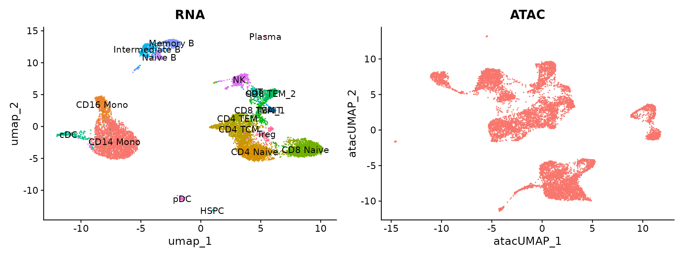
Identifying anchors between scRNA-seq and scATAC-seq datasets
In order to identify ‘anchors’ between scRNA-seq and scATAC-seq
experiments, we first generate a rough estimate of the transcriptional
activity of each gene by quantifying ATAC-seq counts in the 2
kb-upstream region and gene body, using the GeneActivity()
function in the Signac package. The ensuing gene activity scores from
the scATAC-seq data are then used as input for canonical correlation
analysis, along with the gene expression quantifications from scRNA-seq.
We perform this quantification for all genes identified as being highly
variable from the scRNA-seq dataset.
# quantify gene activity
gene.activities <- GeneActivity(pbmc.atac, features = VariableFeatures(pbmc.rna))

# add gene activities as a new assay
pbmc.atac[["ACTIVITY"]] <- CreateAssayObject(counts = gene.activities)

# normalize gene activities
DefaultAssay(pbmc.atac) <- "ACTIVITY"
pbmc.atac <- NormalizeData(pbmc.atac)
pbmc.atac <- ScaleData(pbmc.atac, features = rownames(pbmc.atac))
# Identify anchors
transfer.anchors <- FindTransferAnchors(reference = pbmc.rna, query = pbmc.atac, features = VariableFeatures(object = pbmc.rna),
    reference.assay = "RNA", query.assay = "ACTIVITY", reduction = "cca")
Annotate scATAC-seq cells via label transfer
After identifying anchors, we can transfer annotations from the
scRNA-seq dataset onto the scATAC-seq cells. The annotations are stored
in the seurat_annotations field, and are provided as input
to the refdata parameter. The output will contain a matrix
with predictions and confidence scores for each ATAC-seq cell.
celltype.predictions <- TransferData(anchorset = transfer.anchors, refdata = pbmc.rna$seurat_annotations,
    weight.reduction = pbmc.atac[["lsi"]], dims = 2:30)

pbmc.atac <- AddMetaData(pbmc.atac, metadata = celltype.predictions)
Why do you choose different (non-default) values for reduction and weight.reduction?
In FindTransferAnchors(), we typically project the PCA
structure from the reference onto the query when transferring between
scRNA-seq datasets. However, when transferring across modalities we find
that CCA better captures the shared feature correlation structure and
therefore set reduction = 'cca' here. Additionally, by
default in TransferData() we use the same projected PCA
structure to compute the weights of the local neighborhood of anchors
that influence each cell’s prediction. In the case of scRNA-seq to
scATAC-seq transfer, we use the low dimensional space learned by
computing an LSI on the ATAC-seq data to compute these weights as this
better captures the internal structure of the ATAC-seq data.
After performing transfer, the ATAC-seq cells have predicted
annotations (transferred from the scRNA-seq dataset) stored in the
predicted.id field. Since these cells were measured with
the multiome kit, we also have a ground-truth annotation that can be
used for evaluation. You can see that the predicted and actual
annotations are extremely similar.
pbmc.atac$annotation_correct <- pbmc.atac$predicted.id == pbmc.atac$seurat_annotations
p1 <- DimPlot(pbmc.atac, group.by = "predicted.id", label = TRUE) + NoLegend() + ggtitle("Predicted annotation")
p2 <- DimPlot(pbmc.atac, group.by = "seurat_annotations", label = TRUE) + NoLegend() + ggtitle("Ground-truth annotation")
p1 | p2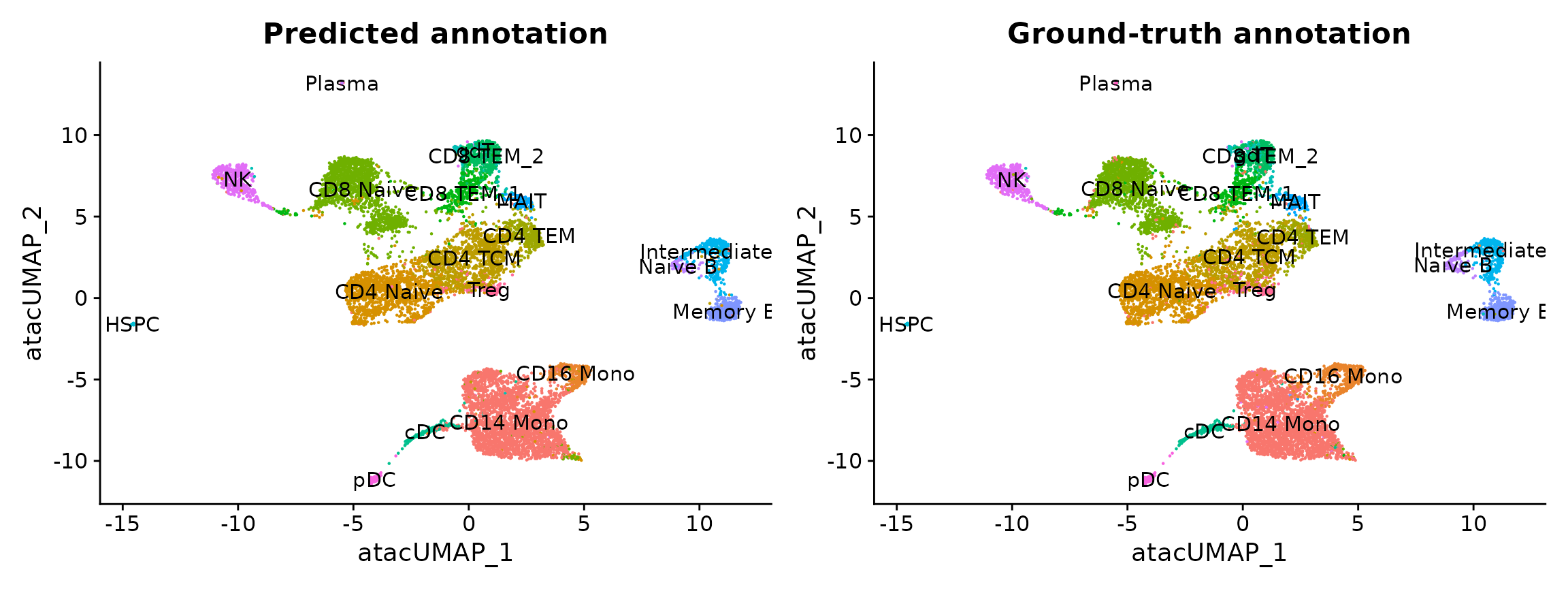
In this example, the annotation for an scATAC-seq profile is
correctly predicted via scRNA-seq integration ~90% of the time. In
addition, the prediction.score.max field quantifies the
uncertainty associated with our predicted annotations. We can see that
cells that are correctly annotated are typically associated with high
prediction scores (>90%), while cells that are incorrectly annotated
are associated with sharply lower prediction scores (<50%). Incorrect
assignments also tend to reflect closely related cell types
(i.e. Intermediate vs. Naive B cells).
predictions <- table(pbmc.atac$seurat_annotations, pbmc.atac$predicted.id)
predictions <- predictions/rowSums(predictions)  # normalize for number of cells in each cell type
predictions <- as.data.frame(predictions)
p1 <- ggplot(predictions, aes(Var1, Var2, fill = Freq)) + geom_tile() + scale_fill_gradient(name = "Fraction of cells",
    low = "#ffffc8", high = "#7d0025") + xlab("Cell type annotation (RNA)") + ylab("Predicted cell type label (ATAC)") +
    theme_cowplot() + theme(axis.text.x = element_text(angle = 90, vjust = 0.5, hjust = 1))

correct <- length(which(pbmc.atac$seurat_annotations == pbmc.atac$predicted.id))
incorrect <- length(which(pbmc.atac$seurat_annotations != pbmc.atac$predicted.id))
data <- FetchData(pbmc.atac, vars = c("prediction.score.max", "annotation_correct"))
p2 <- ggplot(data, aes(prediction.score.max, fill = annotation_correct, colour = annotation_correct)) +
    geom_density(alpha = 0.5) + theme_cowplot() + scale_fill_discrete(name = "Annotation Correct",
    labels = c(paste0("FALSE (n = ", incorrect, ")"), paste0("TRUE (n = ", correct, ")"))) + scale_color_discrete(name = "Annotation Correct",
    labels = c(paste0("FALSE (n = ", incorrect, ")"), paste0("TRUE (n = ", correct, ")"))) + xlab("Prediction Score")
p1 + p2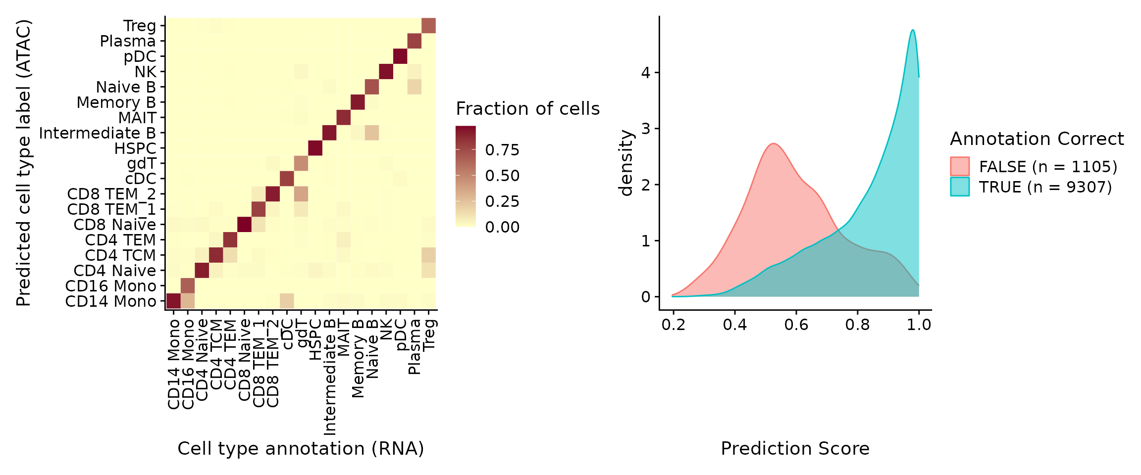
Co-embedding scRNA-seq and scATAC-seq datasets
In addition to transferring labels across modalities, it is also possible to visualize scRNA-seq and scATAC-seq cells on the same plot. We emphasize that this step is primarily for visualization, and is an optional step. Typically, when we perform integrative analysis between scRNA-seq and scATAC-seq datasets, we focus primarily on label transfer as described above. We demonstrate our workflows for co-embedding below, and again highlight that this is for demonstration purposes, especially as in this particular case both the scRNA-seq profiles and scATAC-seq profiles were actually measured in the same cells.
In order to perform co-embedding, we first ‘impute’ RNA expression into the scATAC-seq cells based on the previously computed anchors, and then merge the datasets.
# note that we restrict the imputation to variable genes from scRNA-seq, but could impute the
# full transcriptome if we wanted to
genes.use <- VariableFeatures(pbmc.rna)
refdata <- GetAssayData(pbmc.rna, assay = "RNA", layer = "data")[genes.use, ]

# refdata (input) contains a scRNA-seq expression matrix for the scRNA-seq cells.  imputation
# (output) will contain an imputed scRNA-seq matrix for each of the ATAC cells
imputation <- TransferData(anchorset = transfer.anchors, refdata = refdata, weight.reduction = pbmc.atac[["lsi"]],
    dims = 2:30)
pbmc.atac[["RNA"]] <- imputation

coembed <- merge(x = pbmc.rna, y = pbmc.atac)

# Finally, we run PCA and UMAP on this combined object, to visualize the co-embedding of both
# datasets
coembed <- ScaleData(coembed, features = genes.use, do.scale = FALSE)
coembed <- RunPCA(coembed, features = genes.use, verbose = FALSE)
coembed <- RunUMAP(coembed, dims = 1:30)

DimPlot(coembed, group.by = c("orig.ident", "seurat_annotations"))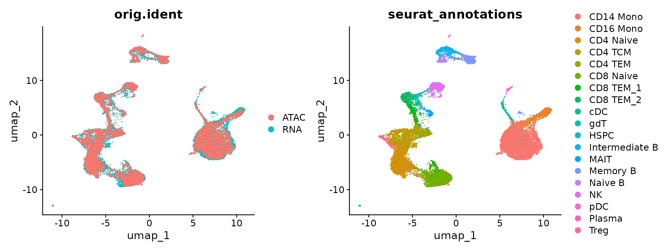
Session Info
## R version 4.5.2 (2025-10-31)
## Platform: x86_64-pc-linux-gnu
## Running under: Ubuntu 24.04.4 LTS
##
## Matrix products: default
## BLAS:   /usr/lib/x86_64-linux-gnu/openblas-pthread/libblas.so.3
## LAPACK: /usr/lib/x86_64-linux-gnu/openblas-pthread/libopenblasp-r0.3.26.so;  LAPACK version 3.12.0
##
## locale:
##  [1] LC_CTYPE=en_US.UTF-8       LC_NUMERIC=C
##  [3] LC_TIME=en_US.UTF-8        LC_COLLATE=en_US.UTF-8
##  [5] LC_MONETARY=en_US.UTF-8    LC_MESSAGES=en_US.UTF-8
##  [7] LC_PAPER=en_US.UTF-8       LC_NAME=C
##  [9] LC_ADDRESS=C               LC_TELEPHONE=C
## [11] LC_MEASUREMENT=en_US.UTF-8 LC_IDENTIFICATION=C
##
## time zone: Etc/UTC
## tzcode source: system (glibc)
##
## attached base packages:
## [1] stats4    stats     graphics  grDevices utils     datasets  methods
## [8] base
##
## other attached packages:
##  [1] future_1.70.0                 cowplot_1.2.0
##  [3] ggplot2_4.0.3                 EnsDb.Hsapiens.v86_2.99.0
##  [5] ensembldb_2.34.0              AnnotationFilter_1.34.0
##  [7] GenomicFeatures_1.62.0        AnnotationDbi_1.72.0
##  [9] Biobase_2.70.0                GenomicRanges_1.62.1
## [11] Seqinfo_1.0.0                 IRanges_2.44.0
## [13] S4Vectors_0.48.1              BiocGenerics_0.56.0
## [15] generics_0.1.4                Signac_1.17.1
## [17] Seurat_5.5.0                  SeuratObject_5.4.0
## [19] sp_2.2-1                      pbmcMultiome.SeuratData_0.1.4
## [21] SeuratData_0.2.2.9002
##
## loaded via a namespace (and not attached):
##   [1] RcppAnnoy_0.0.23            splines_4.5.2
##   [3] later_1.4.8                 BiocIO_1.20.0
##   [5] bitops_1.0-9                tibble_3.3.1
##   [7] polyclip_1.10-7             rpart_4.1.24
##   [9] XML_3.99-0.23               fastDummies_1.7.6
##  [11] lifecycle_1.0.5             globals_0.19.1
##  [13] lattice_0.22-7              MASS_7.3-65
##  [15] backports_1.5.0             magrittr_2.0.5
##  [17] Hmisc_5.2-5                 plotly_4.12.0
##  [19] sass_0.4.10                 rmarkdown_2.30
##  [21] jquerylib_0.1.4             yaml_2.3.12
##  [23] httpuv_1.6.16               otel_0.2.0
##  [25] sctransform_0.4.3           spam_2.11-3
##  [27] spatstat.sparse_3.1-0       reticulate_1.46.0
##  [29] pbapply_1.7-4               DBI_1.3.0
##  [31] RColorBrewer_1.1-3          abind_1.4-8
##  [33] Rtsne_0.17                  purrr_1.2.1
##  [35] biovizBase_1.58.0           RCurl_1.98-1.18
##  [37] nnet_7.3-20                 VariantAnnotation_1.56.0
##  [39] rappdirs_0.3.4              ggrepel_0.9.8
##  [41] irlba_2.3.7                 listenv_0.10.1
##  [43] spatstat.utils_3.2-2        goftest_1.2-3
##  [45] RSpectra_0.16-2             spatstat.random_3.4-5
##  [47] fitdistrplus_1.2-6          parallelly_1.47.0
##  [49] pkgdown_2.2.0               DelayedArray_0.36.1
##  [51] codetools_0.2-20            RcppRoll_0.3.2
##  [53] tidyselect_1.2.1            UCSC.utils_1.6.1
##  [55] farver_2.1.2                base64enc_0.1-6
##  [57] matrixStats_1.5.0           spatstat.explore_3.8-0
##  [59] GenomicAlignments_1.46.0    jsonlite_2.0.0
##  [61] Formula_1.2-5               progressr_0.19.0
##  [63] ggridges_0.5.7              survival_3.8-3
##  [65] systemfonts_1.3.2           tools_4.5.2
##  [67] ragg_1.5.1                  ica_1.0-3
##  [69] Rcpp_1.1.1-1.1              glue_1.8.0
##  [71] SparseArray_1.10.10         gridExtra_2.3
##  [73] xfun_0.56                   MatrixGenerics_1.22.0
##  [75] GenomeInfoDb_1.46.2         dplyr_1.2.0
##  [77] withr_3.0.2                 formatR_1.14
##  [79] fastmap_1.2.0               digest_0.6.39
##  [81] R6_2.6.1                    mime_0.13
##  [83] colorspace_2.1-2            textshaping_1.0.5
##  [85] scattermore_1.2             tensor_1.5.1
##  [87] dichromat_2.0-0.1           spatstat.data_3.1-9
##  [89] RSQLite_2.4.6               cigarillo_1.0.0
##  [91] tidyr_1.3.2                 data.table_1.18.2.1
##  [93] rtracklayer_1.70.1          S4Arrays_1.10.1
##  [95] httr_1.4.8                  htmlwidgets_1.6.4
##  [97] uwot_0.2.4                  pkgconfig_2.0.3
##  [99] gtable_0.3.6                blob_1.3.0
## [101] lmtest_0.9-40               S7_0.2.1
## [103] XVector_0.50.0              htmltools_0.5.9
## [105] dotCall64_1.2               ProtGenerics_1.42.0
## [107] scales_1.4.0                png_0.1-9
## [109] spatstat.univar_3.1-7       rstudioapi_0.18.0
## [111] knitr_1.51                  reshape2_1.4.5
## [113] rjson_0.2.23                checkmate_2.3.4
## [115] nlme_3.1-168                curl_7.0.0
## [117] cachem_1.1.0                zoo_1.8-15
## [119] stringr_1.6.0               KernSmooth_2.23-26
## [121] parallel_4.5.2              miniUI_0.1.2
## [123] foreign_0.8-90              restfulr_0.0.16
## [125] desc_1.4.3                  pillar_1.11.1
## [127] grid_4.5.2                  vctrs_0.7.1
## [129] RANN_2.6.2                  promises_1.5.0
## [131] xtable_1.8-8                cluster_2.1.8.2
## [133] htmlTable_2.5.0             evaluate_1.0.5
## [135] cli_3.6.6                   compiler_4.5.2
## [137] Rsamtools_2.26.0            rlang_1.2.0
## [139] crayon_1.5.3                future.apply_1.20.2
## [141] labeling_0.4.3              plyr_1.8.9
## [143] fs_2.1.0                    stringi_1.8.7
## [145] viridisLite_0.4.3           deldir_2.0-4
## [147] BiocParallel_1.44.0         Biostrings_2.78.0
## [149] lazyeval_0.2.3              spatstat.geom_3.7-3
## [151] Matrix_1.7-5                BSgenome_1.78.0
## [153] RcppHNSW_0.6.0              patchwork_1.3.2
## [155] sparseMatrixStats_1.22.0    bit64_4.6.0-1
## [157] KEGGREST_1.50.0             shiny_1.13.0
## [159] SummarizedExperiment_1.40.0 ROCR_1.0-12
## [161] igraph_2.3.0                memoise_2.0.1
## [163] bslib_0.10.0                fastmatch_1.1-8
## [165] bit_4.6.0