Mixscape Vignette
Compiled: May 01, 2026
Source:vignettes/mixscape_vignette.Rmd
mixscape_vignette.RmdOverview
This tutorial demonstrates how to use mixscape for the analyses of single-cell pooled CRISPR screens. We introduce new Seurat functions for:
- Calculating the perturbation-specific signature of every cell.
- Identifying and removing cells that have ‘escaped’ CRISPR perturbation.
- Visualizing similarities/differences across different perturbations.
Loading required packages
# Load packages.
library(Seurat)
library(SeuratData)
library(ggplot2)
library(patchwork)
library(scales)
library(dplyr)
library(reshape2)

# Download dataset using SeuratData.
InstallData(ds = "thp1.eccite")

# Setup custom theme for plotting.
custom_theme <- theme(
  plot.title = element_text(size=16, hjust = 0.5),
  legend.key.size = unit(0.7, "cm"),
  legend.text = element_text(size = 14))
Loading Seurat object containing ECCITE-seq dataset
We use a 111 gRNA ECCITE-seq dataset generated from stimulated THP-1 cells that was recently published from our lab on bioRxiv Papalexi et al. 2020. This dataset can be easily downloaded from the SeuratData package.
# Load object.
eccite <- LoadData(ds = "thp1.eccite")

# Normalize protein.
eccite <- NormalizeData(
  object = eccite,
  assay = "ADT",
  normalization.method = "CLR",
  margin = 2)
RNA-based clustering is driven by confounding sources of variation
Here, we follow the standard Seurat workflow to cluster cells based on their gene expression profiles. We expected to obtain perturbation-specific clusters; however, we saw that clustering is primarily driven by cell cycle phase and replicate ID. We only observed one perturbation-specific cluster containing cells expressing IFNgamma pathway gRNAs.
# Prepare RNA assay for dimensionality reduction:
# Normalize data, find variable features and scale data.
DefaultAssay(object = eccite) <- 'RNA'
eccite <- NormalizeData(object = eccite) %>% FindVariableFeatures() %>% ScaleData()

# Run Principle Component Analysis (PCA) to reduce the dimensionality of the data.
eccite <- RunPCA(object = eccite)

# Run Uniform Manifold Approximation and Projection (UMAP) to visualize clustering in 2-D.
eccite <- RunUMAP(object = eccite, dims = 1:40)

# Generate plots to check if clustering is driven by biological replicate ID,
# cell cycle phase or target gene class.
p1 <- DimPlot(
  object = eccite,
  group.by = 'replicate',
  label = F,
  pt.size = 0.2,
  reduction = "umap", cols = "Dark2", repel = T) +
  scale_color_brewer(palette = "Dark2") +
  ggtitle("Biological Replicate") +
  xlab("UMAP 1") +
  ylab("UMAP 2") +
  custom_theme

p2 <- DimPlot(
  object = eccite,
  group.by = 'Phase',
  label = F, pt.size = 0.2,
  reduction = "umap", repel = T) +
  ggtitle("Cell Cycle Phase") +
  ylab("UMAP 2") +
  xlab("UMAP 1") +
  custom_theme

p3 <- DimPlot(
  object = eccite,
  group.by = 'crispr',
  pt.size = 0.2,
  reduction = "umap",
  split.by = "crispr",
  ncol = 1,
  cols = c("grey39","goldenrod3")) +
  ggtitle("Perturbation Status") +
  ylab("UMAP 2") +
  xlab("UMAP 1") +
  custom_theme

# Visualize plots.
((p1 / p2 + plot_layout(guides = 'auto')) | p3 )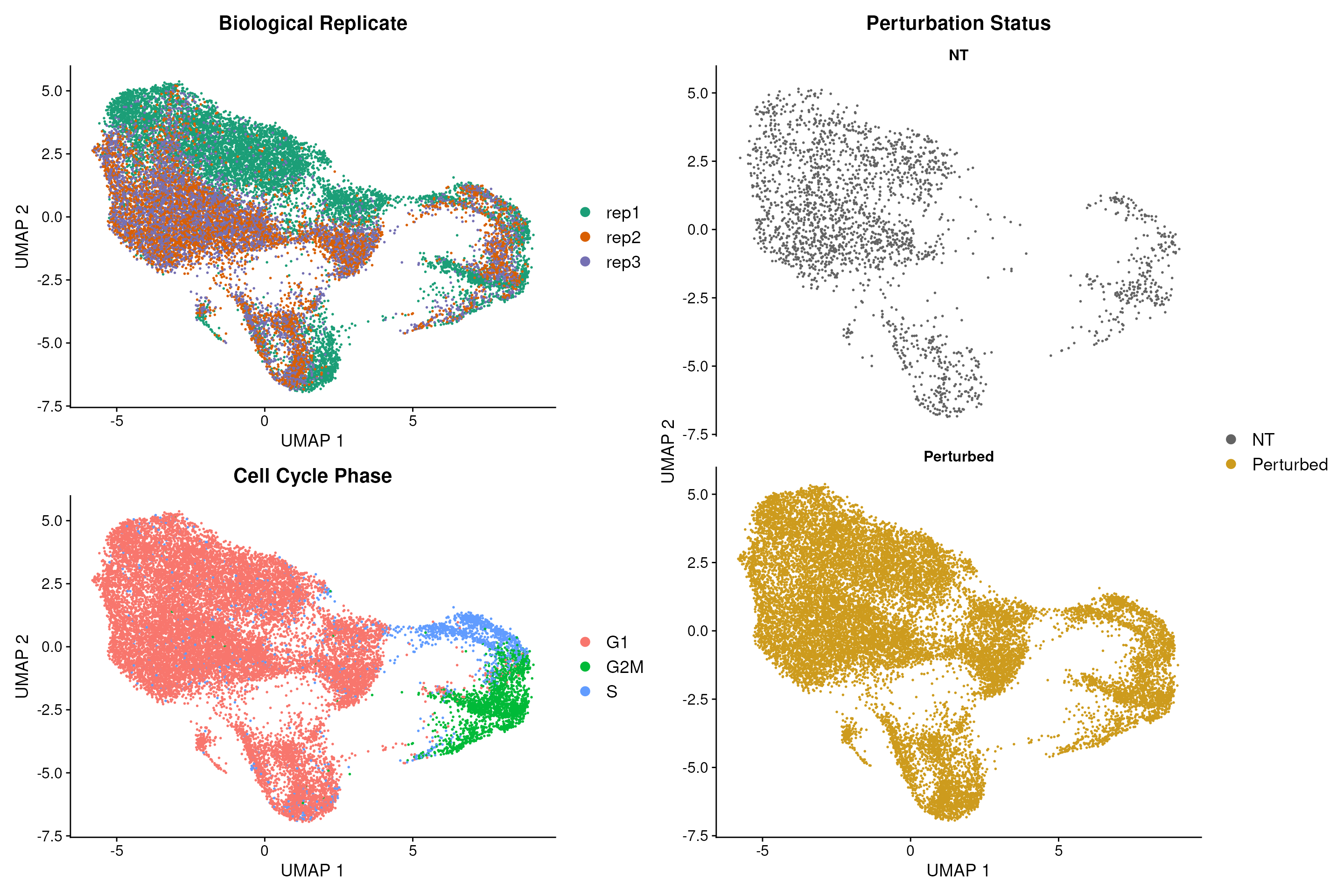
Calculating local perturbation signatures mitigates confounding effects
To calculate local perturbation signatures we set the number of non-targeting Nearest Neighbors (NNs) equal to k=20 and we recommend that the user picks a k from the following range: 20 < k < 30. Intuitively, the user does not want to set k to a very small or large number as this will most likely not remove the technical variation from the dataset. Using the PRTB signature to cluster cells removes all technical variation and reveals one additional perturbation-specific cluster.
# Calculate perturbation signature (PRTB).
eccite<- CalcPerturbSig(
  object = eccite,
  assay = "RNA",
  slot = "data",
  gd.class ="gene",
  nt.cell.class = "NT",
  reduction = "pca",
  ndims = 40,
  num.neighbors = 20,
  split.by = "replicate",
  new.assay.name = "PRTB")

# Prepare PRTB assay for dimensionality reduction:
# Normalize data, find variable features and center data.
DefaultAssay(object = eccite) <- 'PRTB'

# Use variable features from RNA assay.
VariableFeatures(object = eccite) <- VariableFeatures(object = eccite[["RNA"]])
eccite <- ScaleData(object = eccite, do.scale = F, do.center = T)

# Run PCA to reduce the dimensionality of the data.
eccite <- RunPCA(object = eccite, reduction.key = 'prtbpca', reduction.name = 'prtbpca')

# Run UMAP to visualize clustering in 2-D.
eccite <- RunUMAP(
  object = eccite,
  dims = 1:40,
  reduction = 'prtbpca',
  reduction.key = 'prtbumap',
  reduction.name = 'prtbumap')

# Generate plots to check if clustering is driven by biological replicate ID,
# cell cycle phase or target gene class.
q1 <- DimPlot(
  object = eccite,
  group.by = 'replicate',
  reduction = 'prtbumap',
  pt.size = 0.2, cols = "Dark2", label = F, repel = T) +
  scale_color_brewer(palette = "Dark2") +
  ggtitle("Biological Replicate") +
  ylab("UMAP 2") +
  xlab("UMAP 1") +
  custom_theme

q2 <- DimPlot(
  object = eccite,
  group.by = 'Phase',
  reduction = 'prtbumap',
  pt.size = 0.2, label = F, repel = T) +
  ggtitle("Cell Cycle Phase") +
  ylab("UMAP 2") +
  xlab("UMAP 1") +
  custom_theme

q3 <- DimPlot(
  object = eccite,
  group.by = 'crispr',
  reduction = 'prtbumap',
  split.by = "crispr",
  ncol = 1,
  pt.size = 0.2,
  cols = c("grey39","goldenrod3")) +
  ggtitle("Perturbation Status") +
  ylab("UMAP 2") +
  xlab("UMAP 1") +
  custom_theme

# Visualize plots.
(q1 / q2 + plot_layout(guides = 'auto') | q3)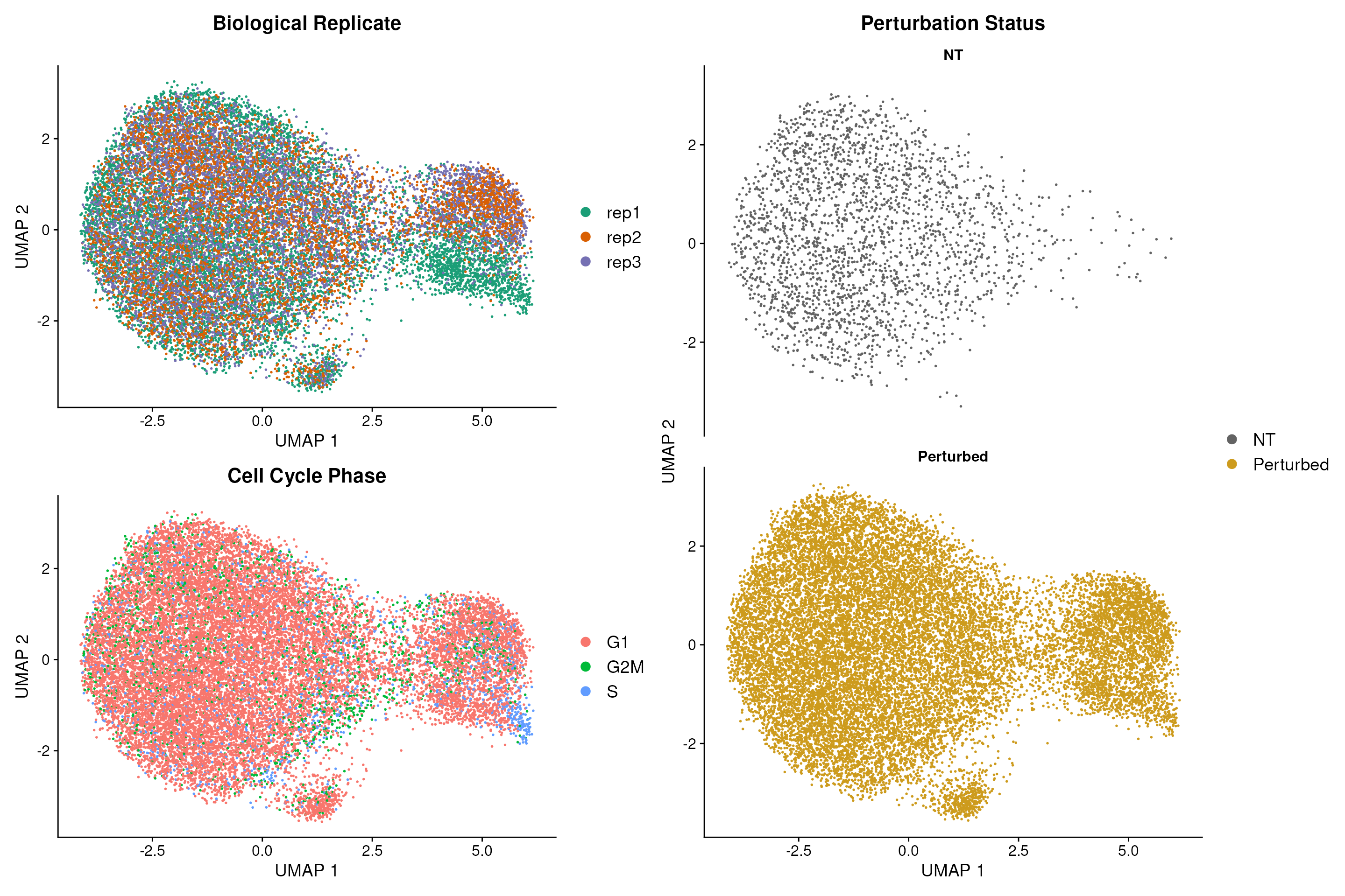
Mixscape identifies cells with no detectable perturbation
Here, we are assuming each target gene class is a mixture of two
Gaussian distributions, one representing the knockout (KO) and the other
the non-perturbed (NP) cells. We further assume that the distribution of
the NP cells is identical to that of cells expressing non-targeting
gRNAs (NT) and we try to estimate the distribution of KO cells using the
function normalmixEM() from the mixtools package. Next, we
calculate the posterior probability that a cell belongs to the KO
distribution and classify cells with a probability higher than 0.5 as
KOs. Applying this method we identify KOs in 11 target gene classes and
detect variation in gRNA targeting efficiency within each class.
# Run mixscape.
eccite <- RunMixscape(
  object = eccite,
  assay = "PRTB",
  slot = "scale.data",
  labels = "gene",
  nt.class.name = "NT",
  min.de.genes = 5,
  iter.num = 10,
  de.assay = "RNA",
  verbose = F,
  prtb.type = "KO")

# Calculate percentage of KO cells for all target gene classes.
df <- prop.table(table(eccite$mixscape_class.global, eccite$NT),2)

df2 <- reshape2::melt(df)
df2$Var2 <- as.character(df2$Var2)
test <- df2[which(df2$Var1 == "KO"),]
test <- test[order(test$value, decreasing = T),]
new.levels <- test$Var2
df2$Var2 <- factor(df2$Var2, levels = new.levels )
df2$Var1 <- factor(df2$Var1, levels = c("NT", "NP", "KO"))
df2$gene <- sapply(as.character(df2$Var2), function(x) strsplit(x, split = "g")[[1]][1])
df2$guide_number <- sapply(as.character(df2$Var2),
                           function(x) strsplit(x, split = "g")[[1]][2])
df3 <- df2[-c(which(df2$gene == "NT")),]

p1 <- ggplot(df3, aes(x = guide_number, y = value*100, fill= Var1)) +
  geom_bar(stat= "identity") +
  theme_classic()+
  scale_fill_manual(values = c("grey49", "grey79","coral1")) +
  ylab("% of cells") +
  xlab("sgRNA")

p1 + theme(axis.text.x = element_text(size = 18, hjust = 1),
           axis.text.y = element_text(size = 18),
           axis.title = element_text(size = 16),
           strip.text = element_text(size=16, face = "bold")) +
  facet_wrap(vars(gene),ncol = 5, scales = "free") +
  labs(fill = "mixscape class") +theme(legend.title = element_text(size = 14),
          legend.text = element_text(size = 12))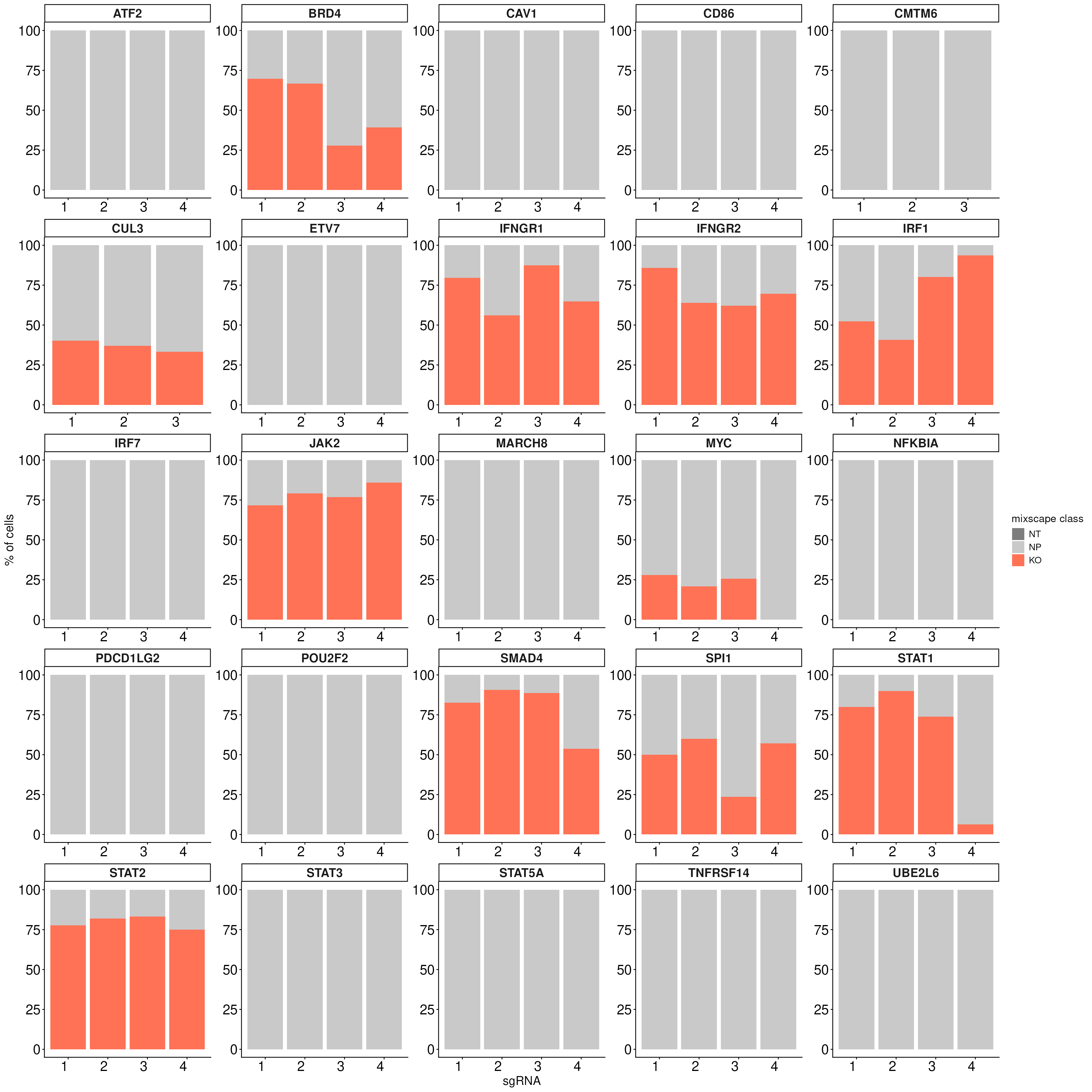
Inspecting mixscape results
To ensure mixscape is assigning the correct perturbation status to cells we can use the functions below to look at the perturbation score distributions and the posterior probabilities of cells within a target gene class (for example IFNGR2) and compare it to those of the NT cells. In addition, we can perform differential expression (DE) analyses and show that only IFNGR2 KO cells have reduced expression of the IFNG-pathway genes. Finally, as an independent check, we can look at the PD-L1 protein expression values in NP and KO cells for target genes known to be PD-L1 regulators.
# Explore the perturbation scores of cells.
PlotPerturbScore(object = eccite,
                 target.gene.ident = "IFNGR2",
                 mixscape.class = "mixscape_class",
                 col = "coral2") +labs(fill = "mixscape class")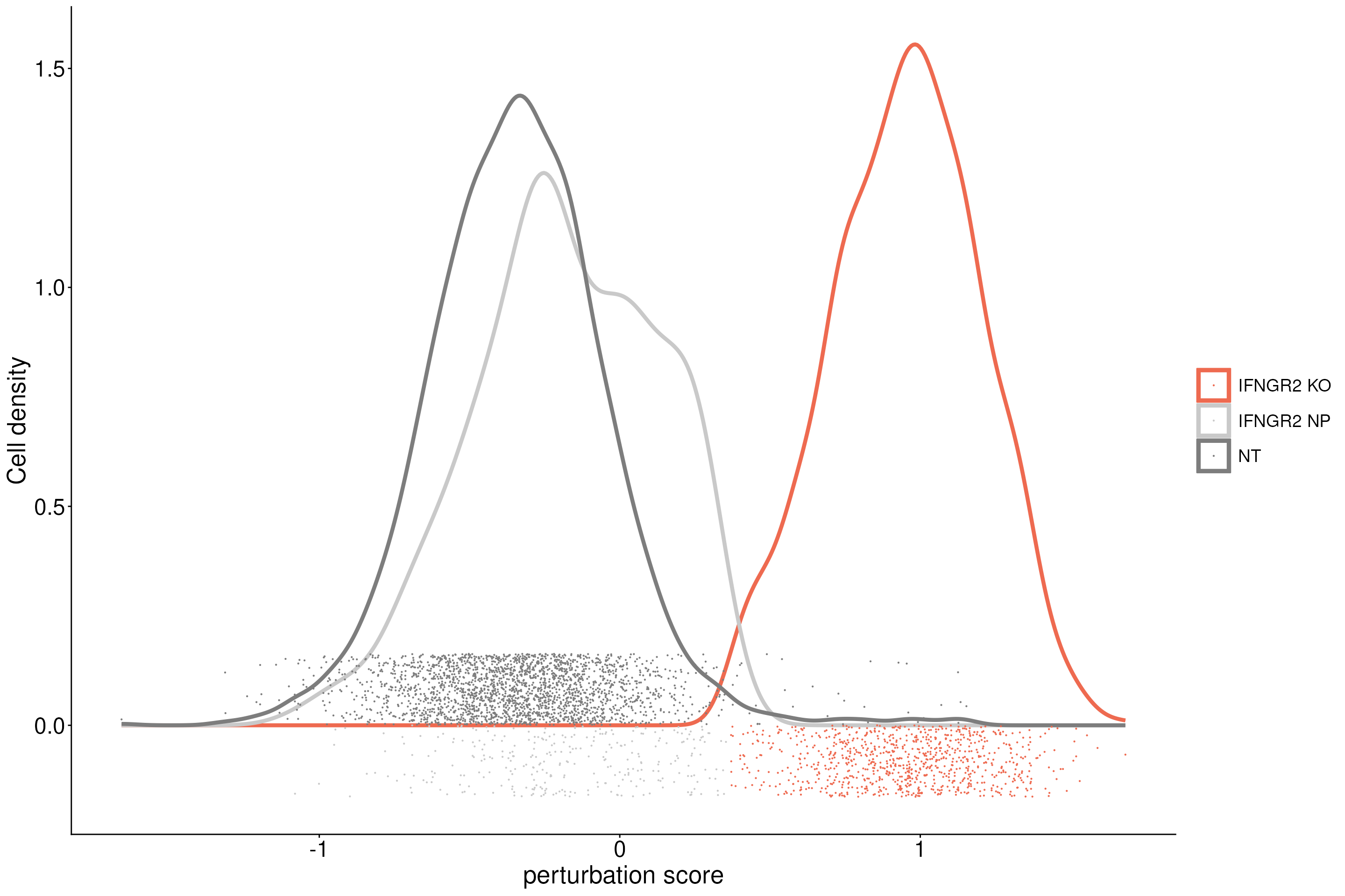
# Inspect the posterior probability values in NP and KO cells.
VlnPlot(eccite, "mixscape_class_p_ko", idents = c("NT", "IFNGR2 KO", "IFNGR2 NP")) +
  theme(axis.text.x = element_text(angle = 0, hjust = 0.5),axis.text = element_text(size = 16) ,plot.title = element_text(size = 20)) +
  NoLegend() +
  ggtitle("mixscape posterior probabilities")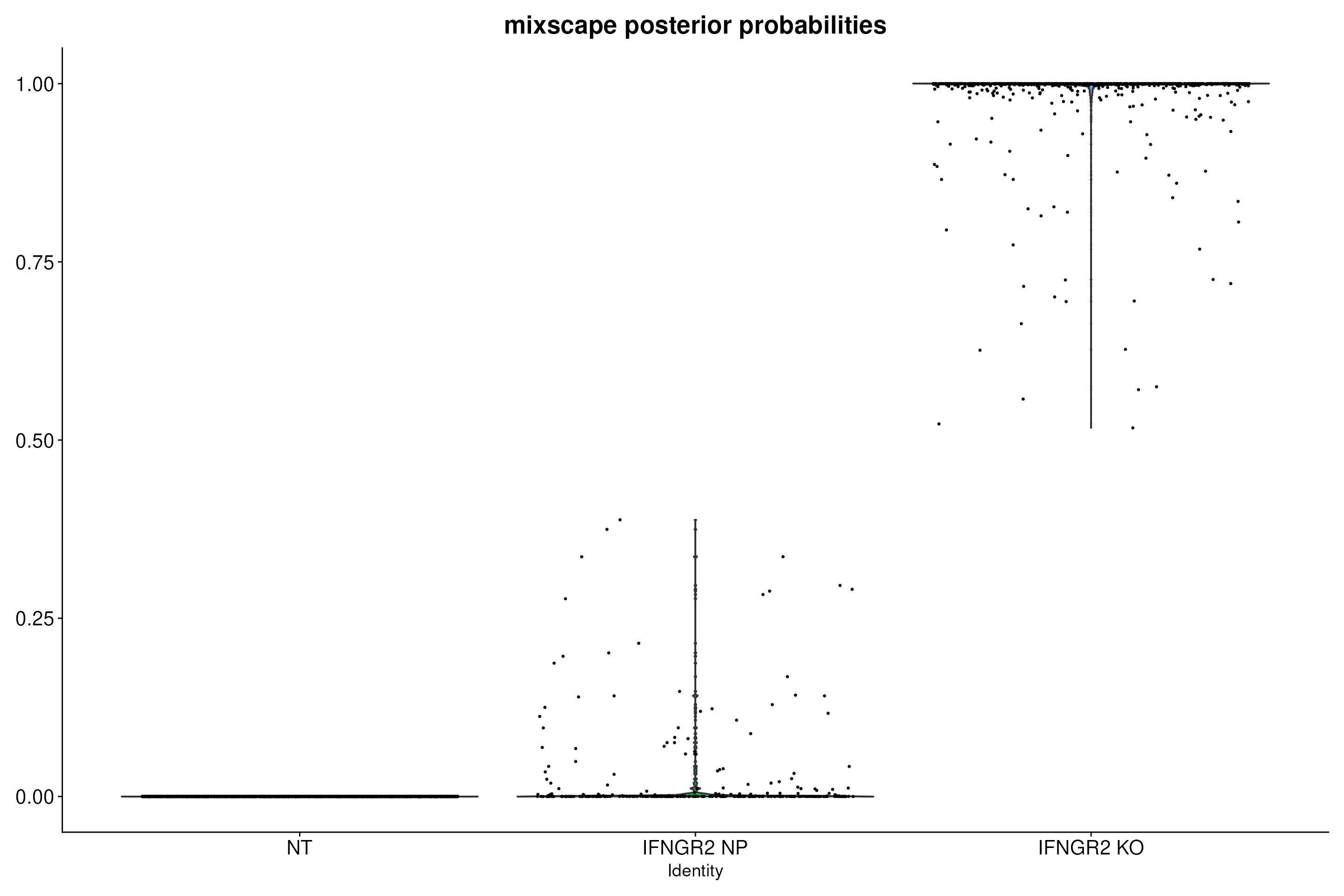
# Run DE analysis and visualize results on a heatmap ordering cells by their posterior
# probability values.
Idents(object = eccite) <- "gene"
MixscapeHeatmap(object = eccite,
                ident.1 = "NT",
                ident.2 = "IFNGR2",
                balanced = F,
                assay = "RNA",
                max.genes = 20, angle = 0,
                group.by = "mixscape_class",
                max.cells.group = 300,
                size=6.5) + NoLegend() +theme(axis.text.y = element_text(size = 16))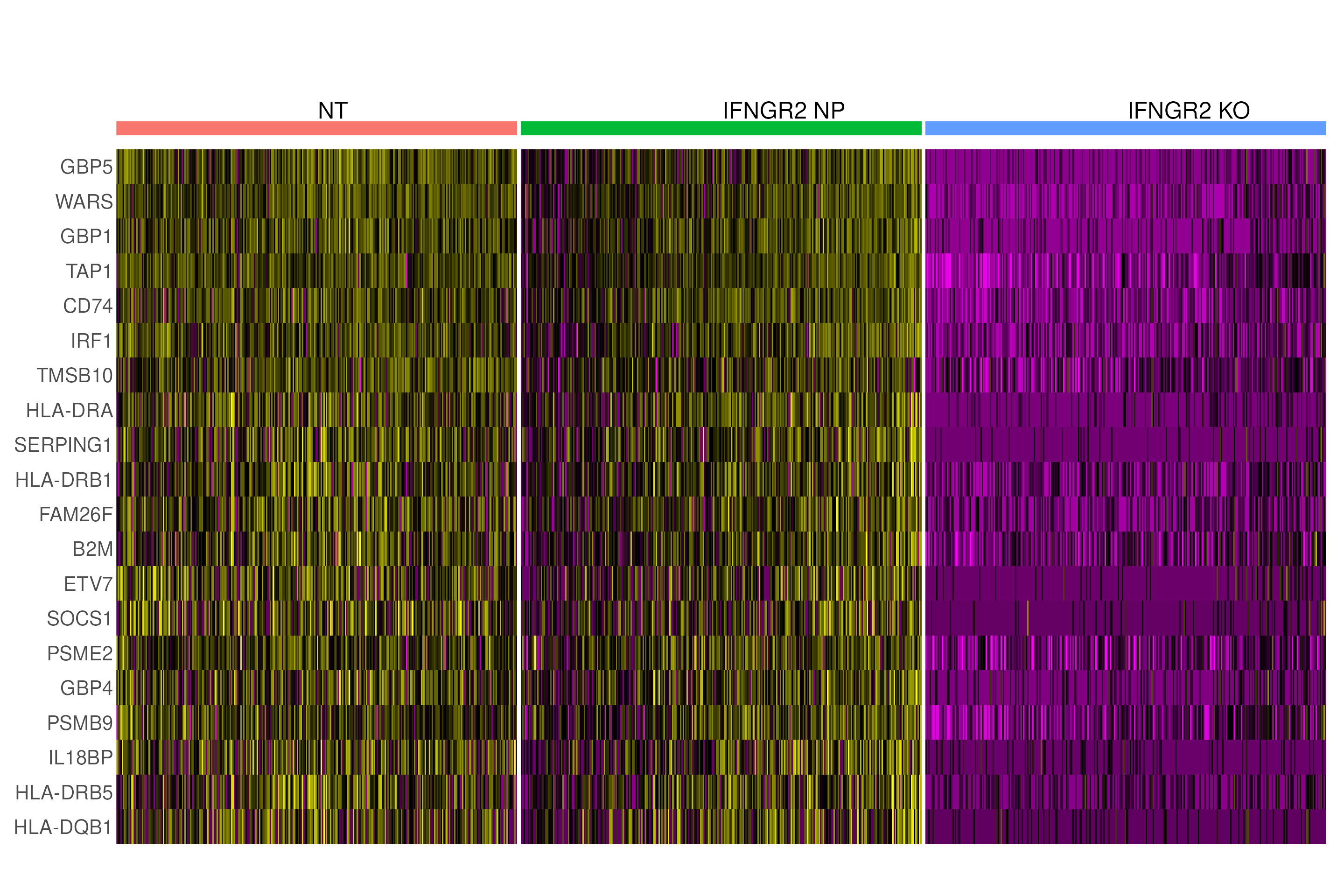
# Show that only IFNG pathway KO cells have a reduction in PD-L1 protein expression.
VlnPlot(
  object = eccite,
  features = "adt_PDL1",
  idents = c("NT","JAK2","STAT1","IFNGR1","IFNGR2", "IRF1"),
  group.by = "gene",
  pt.size = 0.2,
  sort = T,
  split.by = "mixscape_class.global",
  cols = c("coral3","grey79","grey39")) +
  ggtitle("PD-L1 protein") +
  theme(axis.text.x = element_text(angle = 0, hjust = 0.5), plot.title = element_text(size = 20), axis.text = element_text(size = 16))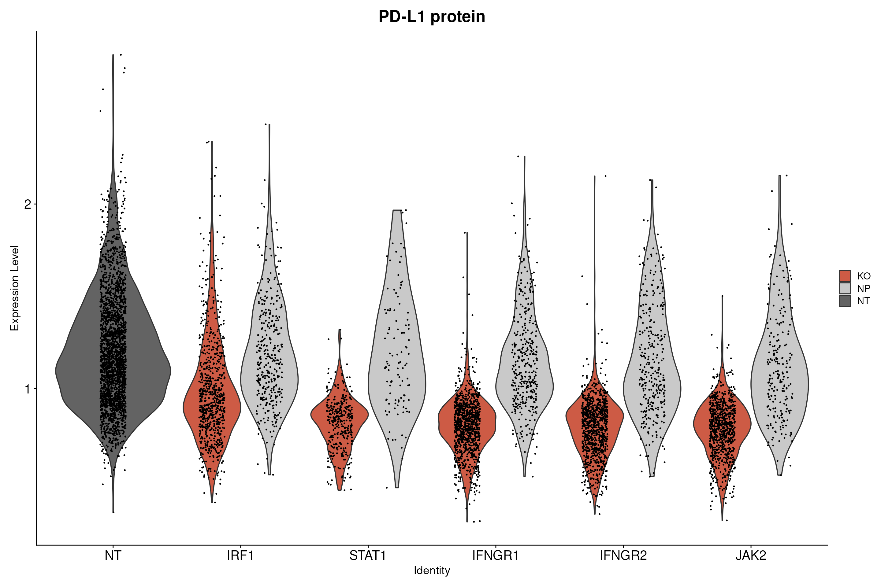
p <- VlnPlot(object = eccite, features = "adt_PDL1", idents = c("NT","JAK2","STAT1","IFNGR1","IFNGR2", "IRF1"), group.by = "gene", pt.size = 0.2, sort = T, split.by = "mixscape_class.global", cols = c("coral3","grey79","grey39")) +ggtitle("PD-L1 protein") +theme(axis.text.x = element_text(angle = 0, hjust = 0.5))Visualizing perturbation responses with Linear Discriminant Analysis (LDA)
We use LDA as a dimensionality reduction method to visualize perturbation-specific clusters. LDA is trying to maximize the separability of known labels (mixscape classes) using both gene expression and the labels as input.
# Remove non-perturbed cells and run LDA to reduce the dimensionality of the data.
Idents(eccite) <- "mixscape_class.global"
sub <- subset(eccite, idents = c("KO", "NT"))

# Run LDA.
sub <- MixscapeLDA(
  object = sub,
  assay = "RNA",
  pc.assay = "PRTB",
  labels = "gene",
  nt.label = "NT",
  npcs = 10,
  logfc.threshold = 0.25,
  verbose = F)

# Use LDA results to run UMAP and visualize cells on 2-D.
# Here, we note that the number of the dimensions to be used is equal to the number of
# labels minus one (to account for NT cells).
sub <- RunUMAP(
  object = sub,
  dims = 1:11,
  reduction = 'lda',
  reduction.key = 'ldaumap',
  reduction.name = 'ldaumap')

# Visualize UMAP clustering results.
Idents(sub) <- "mixscape_class"
sub$mixscape_class <- as.factor(sub$mixscape_class)

# Set colors for each perturbation.
col = setNames(object = hue_pal()(12),nm = levels(sub$mixscape_class))
names(col) <- c(names(col)[1:7], "NT", names(col)[9:12])
col[8] <- "grey39"

p <- DimPlot(object = sub,
             reduction = "ldaumap",
             repel = T,
             label.size = 5,
             label = T,
             cols = col) + NoLegend()

p2 <- p+
  scale_color_manual(values=col, drop=FALSE) +
  ylab("UMAP 2") +
  xlab("UMAP 1") +
  custom_theme
p2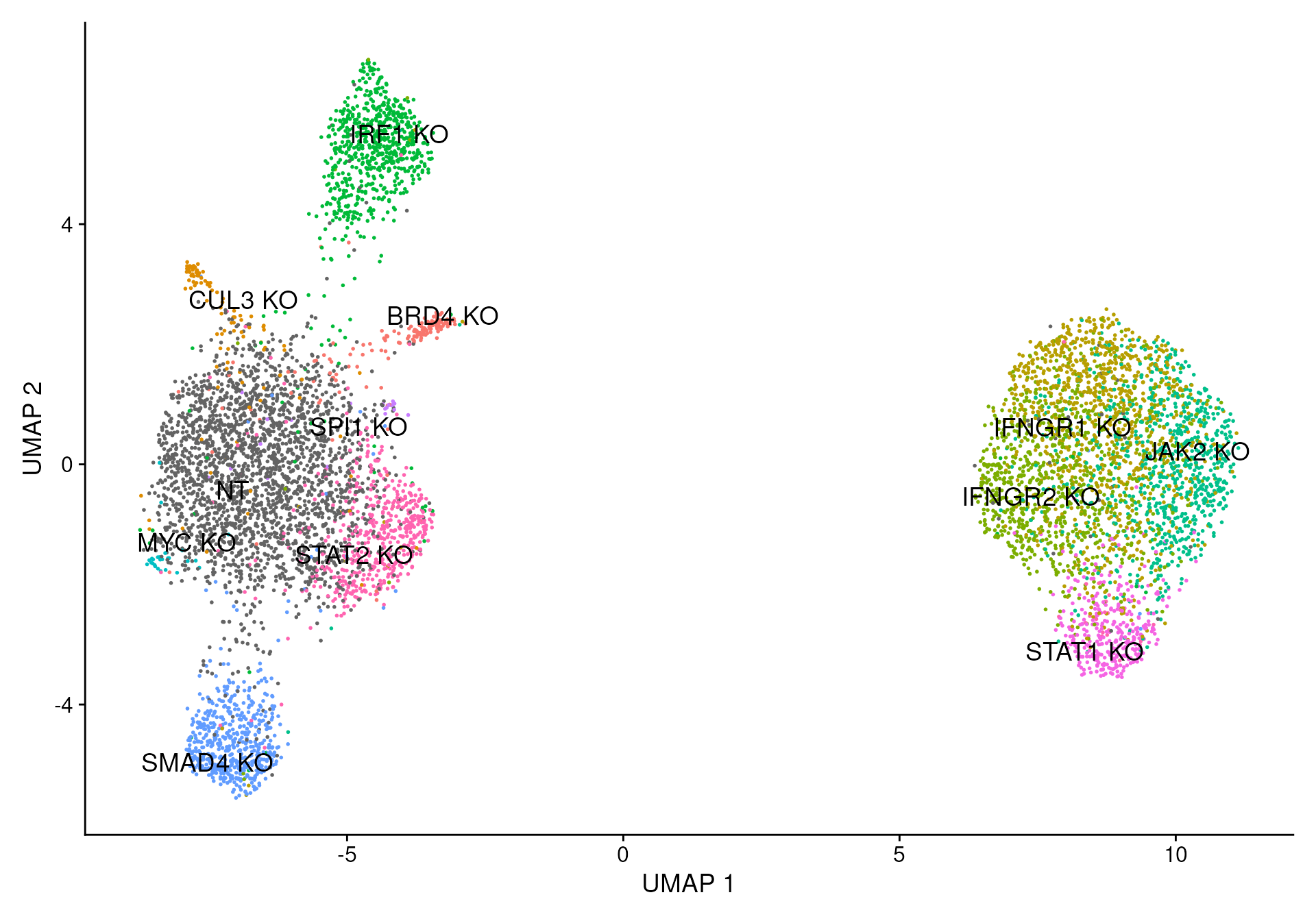
Session Info
## R version 4.5.2 (2025-10-31)
## Platform: x86_64-pc-linux-gnu
## Running under: Ubuntu 24.04.4 LTS
##
## Matrix products: default
## BLAS:   /usr/lib/x86_64-linux-gnu/openblas-pthread/libblas.so.3
## LAPACK: /usr/lib/x86_64-linux-gnu/openblas-pthread/libopenblasp-r0.3.26.so;  LAPACK version 3.12.0
##
## locale:
##  [1] LC_CTYPE=en_US.UTF-8       LC_NUMERIC=C
##  [3] LC_TIME=en_US.UTF-8        LC_COLLATE=en_US.UTF-8
##  [5] LC_MONETARY=en_US.UTF-8    LC_MESSAGES=en_US.UTF-8
##  [7] LC_PAPER=en_US.UTF-8       LC_NAME=C
##  [9] LC_ADDRESS=C               LC_TELEPHONE=C
## [11] LC_MEASUREMENT=en_US.UTF-8 LC_IDENTIFICATION=C
##
## time zone: Etc/UTC
## tzcode source: system (glibc)
##
## attached base packages:
## [1] stats     graphics  grDevices utils     datasets  methods   base
##
## other attached packages:
##  [1] reshape2_1.4.5               dplyr_1.2.0
##  [3] scales_1.4.0                 patchwork_1.3.2
##  [5] ggplot2_4.0.3                thp1.eccite.SeuratData_3.1.5
##  [7] bmcite.SeuratData_0.3.0      SeuratData_0.2.2.9002
##  [9] Seurat_5.5.0                 SeuratObject_5.4.0
## [11] sp_2.2-1
##
## loaded via a namespace (and not attached):
##   [1] RColorBrewer_1.1-3     jsonlite_2.0.0         magrittr_2.0.5
##   [4] ggbeeswarm_0.7.3       spatstat.utils_3.2-2   farver_2.1.2
##   [7] rmarkdown_2.30         fs_2.1.0               ragg_1.5.1
##  [10] vctrs_0.7.1            ROCR_1.0-12            spatstat.explore_3.8-0
##  [13] htmltools_0.5.9        sass_0.4.10            sctransform_0.4.3
##  [16] parallelly_1.47.0      KernSmooth_2.23-26     bslib_0.10.0
##  [19] htmlwidgets_1.6.4      desc_1.4.3             ica_1.0-3
##  [22] plyr_1.8.9             plotly_4.12.0          zoo_1.8-15
##  [25] cachem_1.1.0           igraph_2.3.0           mime_0.13
##  [28] lifecycle_1.0.5        pkgconfig_2.0.3        Matrix_1.7-5
##  [31] R6_2.6.1               fastmap_1.2.0          fitdistrplus_1.2-6
##  [34] future_1.70.0          shiny_1.13.0           digest_0.6.39
##  [37] tensor_1.5.1           RSpectra_0.16-2        irlba_2.3.7
##  [40] textshaping_1.0.5      labeling_0.4.3         progressr_0.19.0
##  [43] spatstat.sparse_3.1-0  httr_1.4.8             polyclip_1.10-7
##  [46] abind_1.4-8            compiler_4.5.2         withr_3.0.2
##  [49] S7_0.2.1               fastDummies_1.7.6      MASS_7.3-65
##  [52] rappdirs_0.3.4         tools_4.5.2            vipor_0.4.7
##  [55] lmtest_0.9-40          otel_0.2.0             beeswarm_0.4.0
##  [58] httpuv_1.6.16          future.apply_1.20.2    goftest_1.2-3
##  [61] glue_1.8.0             nlme_3.1-168           promises_1.5.0
##  [64] grid_4.5.2             Rtsne_0.17             cluster_2.1.8.2
##  [67] generics_0.1.4         gtable_0.3.6           spatstat.data_3.1-9
##  [70] tidyr_1.3.2            data.table_1.18.2.1    spatstat.geom_3.7-3
##  [73] RcppAnnoy_0.0.23       ggrepel_0.9.8          RANN_2.6.2
##  [76] pillar_1.11.1          stringr_1.6.0          limma_3.66.0
##  [79] spam_2.11-3            RcppHNSW_0.6.0         later_1.4.8
##  [82] splines_4.5.2          lattice_0.22-7         survival_3.8-3
##  [85] deldir_2.0-4           tidyselect_1.2.1       miniUI_0.1.2
##  [88] pbapply_1.7-4          knitr_1.51             gridExtra_2.3
##  [91] scattermore_1.2        xfun_0.56              mixtools_2.0.0.1
##  [94] statmod_1.5.1          matrixStats_1.5.0      stringi_1.8.7
##  [97] lazyeval_0.2.3         yaml_2.3.12            evaluate_1.0.5
## [100] codetools_0.2-20       kernlab_0.9-33         tibble_3.3.1
## [103] cli_3.6.6              uwot_0.2.4             xtable_1.8-8
## [106] reticulate_1.46.0      systemfonts_1.3.2      segmented_2.2-1
## [109] jquerylib_0.1.4        Rcpp_1.1.1-1.1         globals_0.19.1
## [112] spatstat.random_3.4-5  png_0.1-9              ggrastr_1.0.2
## [115] spatstat.univar_3.1-7  parallel_4.5.2         pkgdown_2.2.0
## [118] presto_1.0.0           dotCall64_1.2          listenv_0.10.1
## [121] viridisLite_0.4.3      ggridges_0.5.7         purrr_1.2.1
## [124] crayon_1.5.3           rlang_1.2.0            cowplot_1.2.0