Weighted Nearest Neighbor Analysis
Compiled: May 13, 2026
Source:vignettes/weighted_nearest_neighbor_analysis.Rmd
weighted_nearest_neighbor_analysis.RmdThe simultaneous measurement of multiple modalities, known as multimodal analysis, represents an exciting frontier for single-cell genomics and necessitates new computational methods that can define cellular states based on multiple data types. The varying information content of each modality, even across cells in the same dataset, represents a pressing challenge for the analysis and integration of multimodal datasets. In (Hao*, Hao* et al, Cell 2021), we introduce ‘weighted-nearest neighbor’ (WNN) analysis, an unsupervised framework to learn the relative utility of each data type in each cell, enabling an integrative analysis of multiple modalities.
This vignette introduces the WNN workflow for the analysis of multimodal single-cell datasets. The workflow consists of three steps
- Independent preprocessing and dimensional reduction of each modality individually
- Learning cell-specific modality ‘weights’, and constructing a WNN graph that integrates the modalities
- Downstream analysis (i.e. visualization, clustering, etc.) of the WNN graph
We demonstrate the use of WNN analysis on two single-cell multimodal technologies: CITE-seq and 10x multiome. We define the cellular states based on both modalities, instead of either individual modality.
WNN analysis of CITE-seq, RNA + ADT
We use the CITE-seq dataset from (Stuart*, Butler* et al, Cell 2019), which consists of 30,672 scRNA-seq profiles measured alongside a panel of 25 antibodies from bone marrow. The object contains two assays, RNA and antibody-derived tags (ADT).
To run this vignette please install SeuratData, available on GitHub.
InstallData("bmcite")
bm <- LoadData(ds = "bmcite")
We first perform pre-processing and dimensional reduction on both assays independently. We use standard normalization, but you can also use SCTransform or any alternative method.
DefaultAssay(bm) <- 'RNA'
bm <- NormalizeData(bm) %>% FindVariableFeatures() %>% ScaleData() %>% RunPCA()

DefaultAssay(bm) <- 'ADT'
# we will use all ADT features for dimensional reduction
# we set a dimensional reduction name to avoid overwriting the default PCA
VariableFeatures(bm) <- rownames(bm[["ADT"]])
bm <- NormalizeData(bm, normalization.method = 'CLR', margin = 2) %>%
  ScaleData() %>% RunPCA(reduction.name = 'apca')
For each cell, we calculate its closest neighbors in the dataset based on a weighted combination of RNA and protein similarities. The cell-specific modality weights and multimodal neighbors are calculated in a single function, which takes ~2 minutes to run on this dataset. We specify the dimensionality of each modality (similar to specifying the number of PCs to include in scRNA-seq clustering), but you can vary these settings to see that small changes have minimal effect on the overall results.
# Identify multimodal neighbors. These will be stored in the neighbors slot,
# and can be accessed using bm[['weighted.nn']]
# The WNN graph can be accessed at bm[["wknn"]],
# and the SNN graph used for clustering at bm[["wsnn"]]
# Cell-specific modality weights can be accessed at bm$RNA.weight
bm <- FindMultiModalNeighbors(
  bm, reduction.list = list("pca", "apca"),
  dims.list = list(1:30, 1:18), modality.weight.name = "RNA.weight"
)
We can now use these results for downstream analysis, such as visualization and clustering. For example, we can create a UMAP visualization of the data based on a weighted combination of RNA and protein data. We can also perform graph-based clustering and visualize these results on the UMAP, alongside a set of cell annotations.
bm <- RunUMAP(bm, nn.name = "weighted.nn", reduction.name = "wnn.umap", reduction.key = "wnnUMAP_")
bm <- FindClusters(bm, graph.name = "wsnn", algorithm = 3, resolution = 2, verbose = FALSE)
p1 <- DimPlot(bm, reduction = 'wnn.umap', label = TRUE, repel = TRUE, label.size = 2.5) + NoLegend()
p2 <- DimPlot(bm, reduction = 'wnn.umap', group.by = 'celltype.l2', label = TRUE, repel = TRUE, label.size = 2.5) + NoLegend()
p1 + p2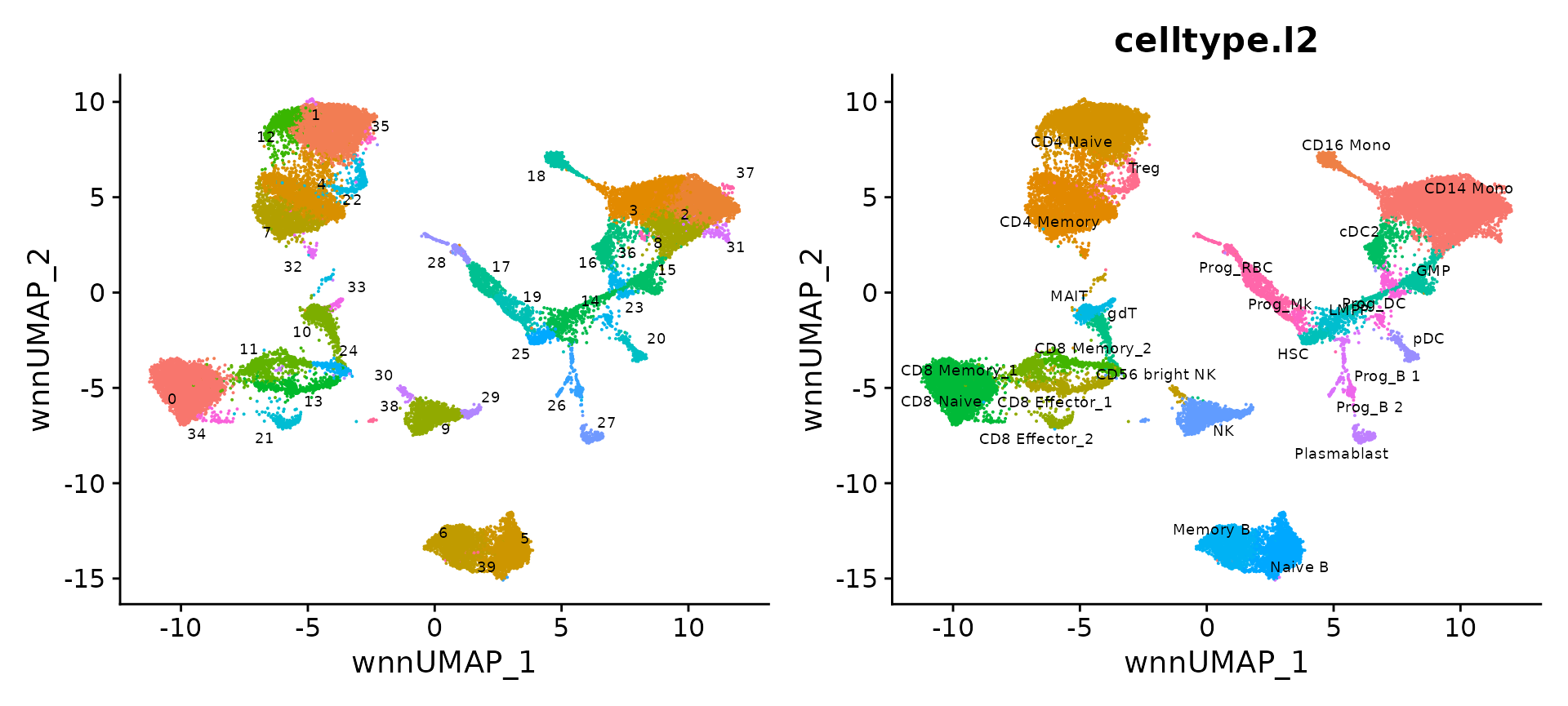
We can also compute UMAP visualization based on only the RNA and protein data and compare. We find that the RNA analysis is more informative than the ADT analysis in identifying progenitor states (the ADT panel contains markers for differentiated cells), while the converse is true of T cell states (where the ADT analysis outperforms RNA).
bm <- RunUMAP(bm, reduction = 'pca', dims = 1:30, assay = 'RNA',
              reduction.name = 'rna.umap', reduction.key = 'rnaUMAP_')
bm <- RunUMAP(bm, reduction = 'apca', dims = 1:18, assay = 'ADT',
              reduction.name = 'adt.umap', reduction.key = 'adtUMAP_')
p3 <- DimPlot(bm, reduction = 'rna.umap', group.by = 'celltype.l2', label = TRUE,
              repel = TRUE, label.size = 2.5) + NoLegend()
p4 <- DimPlot(bm, reduction = 'adt.umap', group.by = 'celltype.l2', label = TRUE,
              repel = TRUE, label.size = 2.5) + NoLegend()
p3 + p4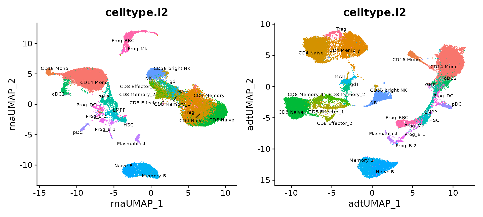
We can visualize the expression of canonical marker genes and proteins on the multimodal UMAP, which can assist in verifying the provided annotations:
p5 <- FeaturePlot(bm, features = c("adt_CD45RA","adt_CD16","adt_CD161"),
                  reduction = 'wnn.umap', max.cutoff = 2,
                  cols = c("lightgrey","darkgreen"), ncol = 3)
p6 <- FeaturePlot(bm, features = c("rna_TRDC","rna_MPO","rna_AVP"),
                  reduction = 'wnn.umap', max.cutoff = 3, ncol = 3)
p5 / p6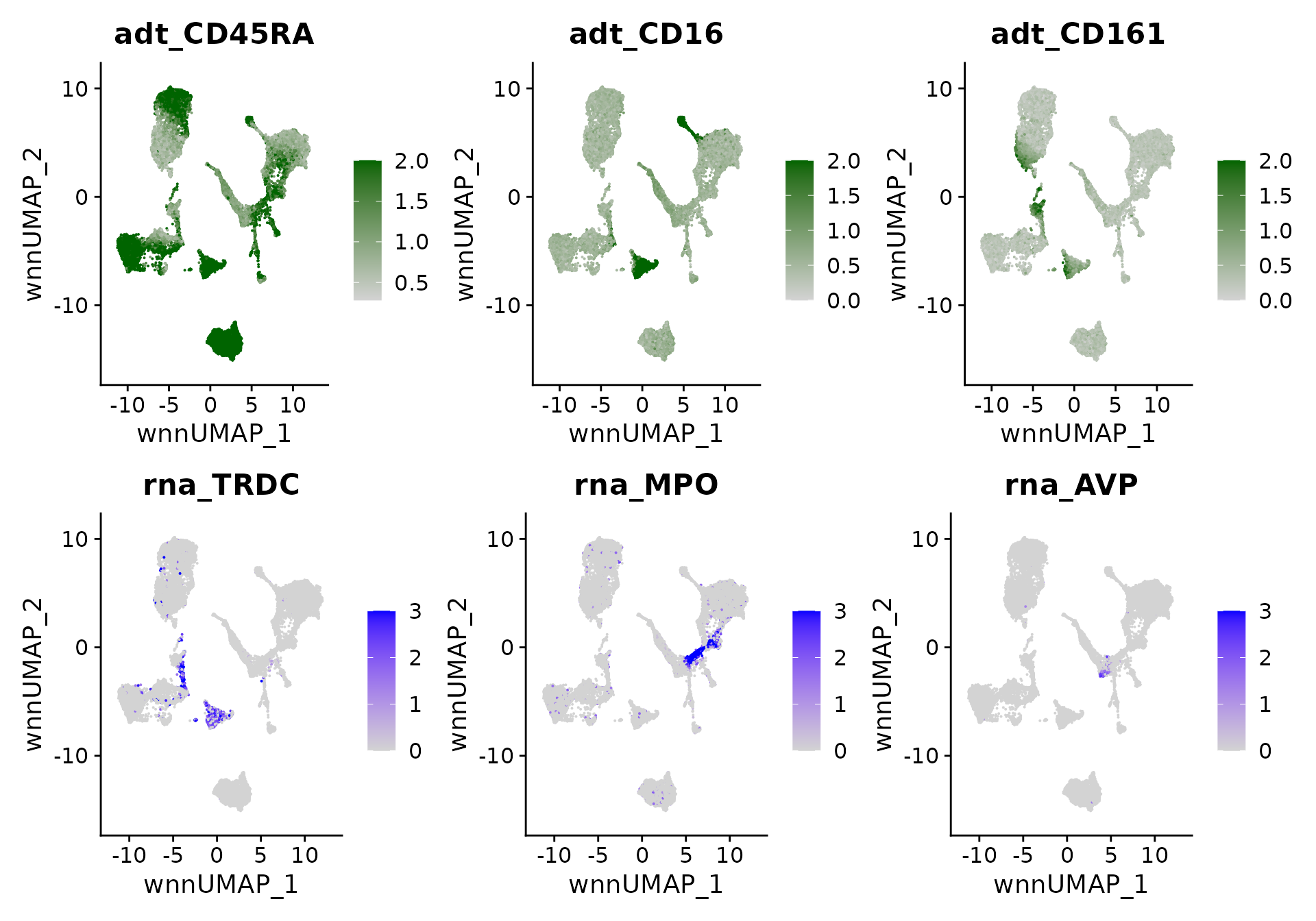
Finally, we can visualize the modality weights that were learned for each cell. Each of the populations with the highest RNA weights represent progenitor cells, while the populations with the highest protein weights represent T cells. This is in line with our biological expectations, as the antibody panel does not contain markers that can distinguish between different progenitor populations.
 VlnPlot(bm, features = "RNA.weight", group.by = 'celltype.l2', sort = TRUE, pt.size = 0.1) +
  NoLegend()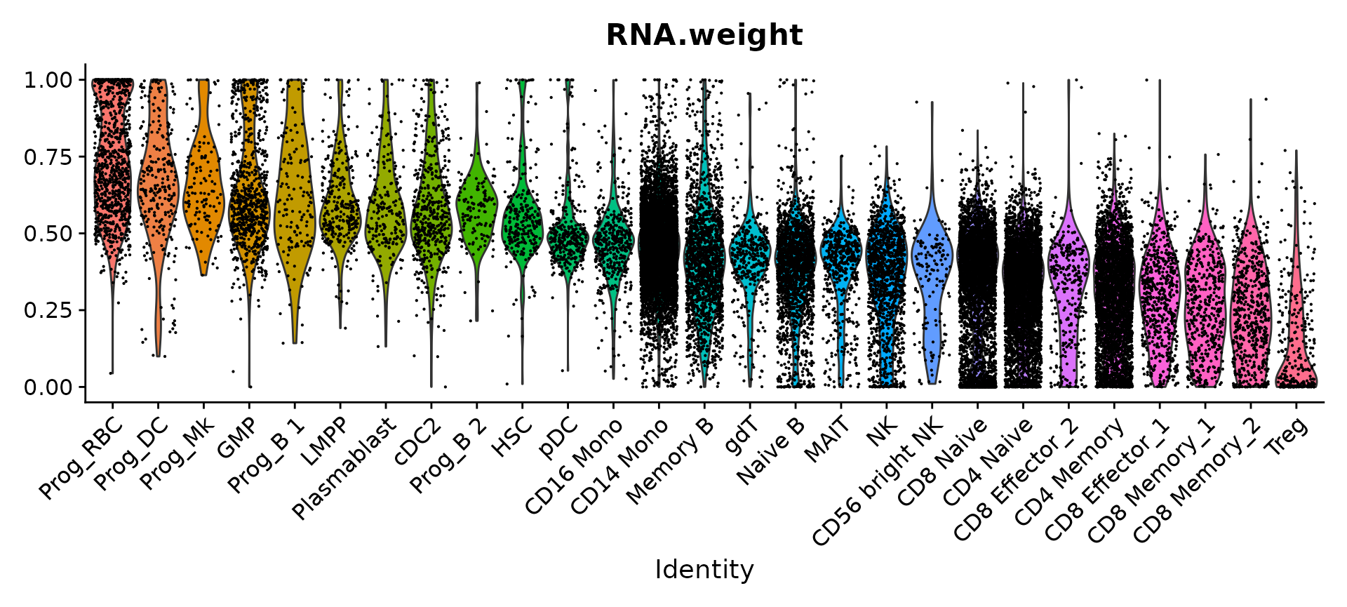
WNN analysis of 10x Multiome, RNA + ATAC
Here, we demonstrate the use of WNN analysis on a second multimodal technology, the 10x multiome RNA+ATAC kit. We use a dataset that is publicly available on the 10x website, where paired transcriptomes and ATAC-seq profiles are measured in 10,412 PBMCs.
We use the same WNN methods as we use in the previous tab, where we apply integrated multimodal analysis to a CITE-seq dataset. In this example we will demonstrate how to:
- Create a multimodal Seurat object with paired transcriptome and ATAC-seq profiles
- Perform weighted neighbor clustering on RNA+ATAC data in single cells
- Leverage both modalities to identify putative regulators of different cell types and states
You can download the dataset from the 10x Genomics website here. Please make sure to download the following files:
- Filtered feature barcode matrix (HDF5)
- ATAC Per fragment information file (TSV.GZ)
- ATAC Per fragment information index (TSV.GZ index)
Finally, in order to run the vignette, make sure the following packages are installed:
- Seurat
- Signac for the analysis of single-cell chromatin datasets
- EnsDb.Hsapiens.v86 for a set of annotations for hg38
- dplyr to help manipulate data tables
library(Seurat)
library(Signac)
library(EnsDb.Hsapiens.v86)
library(dplyr)
library(ggplot2)
library(GenomeInfoDb)
We’ll create a Seurat object based on the gene expression data, and then add in the ATAC-seq data as a second assay. You can explore the Signac getting started vignette for more information on the creation and processing of a ChromatinAssay object.
# the 10x hdf5 file contains both data types.
inputdata.10x <- Read10X_h5("/brahms/choudharys/github/signac/vignette_data/multiomic/pbmc_granulocyte_sorted_10k_filtered_feature_bc_matrix.h5")

# extract RNA and ATAC data
rna_counts <- inputdata.10x$`Gene Expression`
atac_counts <- inputdata.10x$Peaks

# Create Seurat object
pbmc <- CreateSeuratObject(counts = rna_counts)
pbmc[["percent.mt"]] <- PercentageFeatureSet(pbmc, pattern = "^MT-")

# Now add in the ATAC-seq data
# we'll only use peaks in standard chromosomes
grange.counts <- StringToGRanges(rownames(atac_counts), sep = c(":", "-"))
grange.use <- seqnames(grange.counts) %in% standardChromosomes(grange.counts)
atac_counts <- atac_counts[as.vector(grange.use), ]
annotations <- GetGRangesFromEnsDb(ensdb = EnsDb.Hsapiens.v86)
seqlevelsStyle(annotations) <- 'UCSC'
genome(annotations) <- "hg38"

frag.file <- "/brahms/choudharys/github/signac/vignette_data/multiomic/pbmc_granulocyte_sorted_10k_atac_fragments.tsv.gz"
chrom_assay <- CreateChromatinAssay(
   counts = atac_counts,
   sep = c(":", "-"),
   genome = 'hg38',
   fragments = frag.file,
   min.cells = 10,
   annotation = annotations
 )
pbmc[["ATAC"]] <- chrom_assay
We perform basic QC based on the number of detected molecules for each modality as well as mitochondrial percentage.
VlnPlot(pbmc, features = c("nCount_ATAC", "nCount_RNA", "percent.mt"), ncol = 3,
  log = TRUE, pt.size = 0) + NoLegend()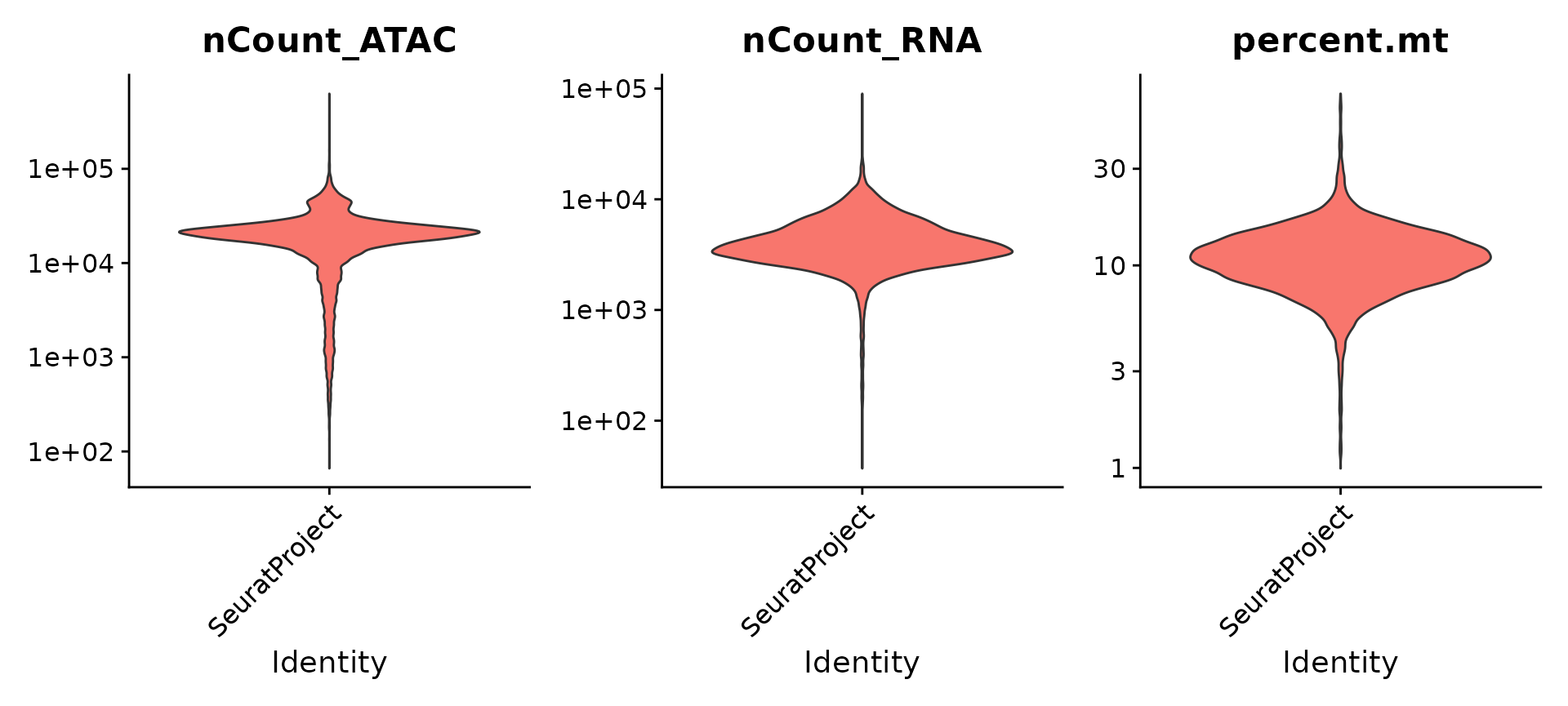
pbmc <- subset(
  x = pbmc,
  subset = nCount_ATAC < 7e4 &
    nCount_ATAC > 5e3 &
    nCount_RNA < 25000 &
    nCount_RNA > 1000 &
    percent.mt < 20
)
We next perform pre-processing and dimensional reduction on both assays independently, using standard approaches for RNA and ATAC-seq data.
# RNA analysis
DefaultAssay(pbmc) <- "RNA"
pbmc <- SCTransform(pbmc, verbose = FALSE) %>% RunPCA() %>% RunUMAP(dims = 1:50, reduction.name = 'umap.rna', reduction.key = 'rnaUMAP_')

# ATAC analysis
# We exclude the first dimension as this is typically correlated with sequencing depth
DefaultAssay(pbmc) <- "ATAC"
pbmc <- RunTFIDF(pbmc)
pbmc <- FindTopFeatures(pbmc, min.cutoff = 'q0')
pbmc <- RunSVD(pbmc)
pbmc <- RunUMAP(pbmc, reduction = 'lsi', dims = 2:50, reduction.name = "umap.atac", reduction.key = "atacUMAP_")
We calculate a WNN graph, representing a weighted combination of RNA and ATAC-seq modalities. We use this graph for UMAP visualization and clustering.
pbmc <- FindMultiModalNeighbors(pbmc, reduction.list = list("pca", "lsi"), dims.list = list(1:50, 2:50))
pbmc <- RunUMAP(pbmc, nn.name = "weighted.nn", reduction.name = "wnn.umap", reduction.key = "wnnUMAP_")
pbmc <- FindClusters(pbmc, graph.name = "wsnn", algorithm = 3, verbose = FALSE)
We annotate the clusters below. Note that you could also annotate the dataset using our supervised mapping pipelines, using either our vignette, or automated web tool, Azimuth.
# perform sub-clustering on cluster 6 to find additional structure
pbmc <- FindSubCluster(pbmc, cluster = 6, graph.name = "wsnn", algorithm = 3)
Idents(pbmc) <- "sub.cluster"
# add annotations
pbmc <- RenameIdents(pbmc, '19' = 'pDC','20' = 'HSPC','15' = 'cDC')
pbmc <- RenameIdents(pbmc, '0' = 'CD14 Mono', '9' ='CD14 Mono', '5' = 'CD16 Mono')
pbmc <- RenameIdents(pbmc, '10' = 'Naive B', '11' = 'Intermediate B', '17' = 'Memory B', '21' = 'Plasma')
pbmc <- RenameIdents(pbmc, '7' = 'NK')
pbmc <- RenameIdents(pbmc, '4' = 'CD4 TCM', '13'= "CD4 TEM", '3' = "CD4 TCM", '16' ="Treg", '1' ="CD4 Naive", '14' = "CD4 Naive")
pbmc <- RenameIdents(pbmc, '2' = 'CD8 Naive', '8'= "CD8 Naive", '12' = 'CD8 TEM_1', '6_0' = 'CD8 TEM_2', '6_1' ='CD8 TEM_2', '6_4' ='CD8 TEM_2')
pbmc <- RenameIdents(pbmc, '18' = 'MAIT')
pbmc <- RenameIdents(pbmc, '6_2' ='gdT', '6_3' = 'gdT')
pbmc$celltype <- Idents(pbmc)
We can visualize clustering based on gene expression, ATAC-seq, or WNN analysis. The differences are more subtle than in the previous analysis (you can explore the weights, which are more evenly split than in our CITE-seq example), but we find that WNN provides the clearest separation of cell states.
p1 <- DimPlot(pbmc, reduction = "umap.rna", group.by = "celltype", label = TRUE, label.size = 2.5, repel = TRUE) + ggtitle("RNA")
p2 <- DimPlot(pbmc, reduction = "umap.atac", group.by = "celltype", label = TRUE, label.size = 2.5, repel = TRUE) + ggtitle("ATAC")
p3 <- DimPlot(pbmc, reduction = "wnn.umap", group.by = "celltype", label = TRUE, label.size = 2.5, repel = TRUE) + ggtitle("WNN")
p1 + p2 + p3 & NoLegend() & theme(plot.title = element_text(hjust = 0.5))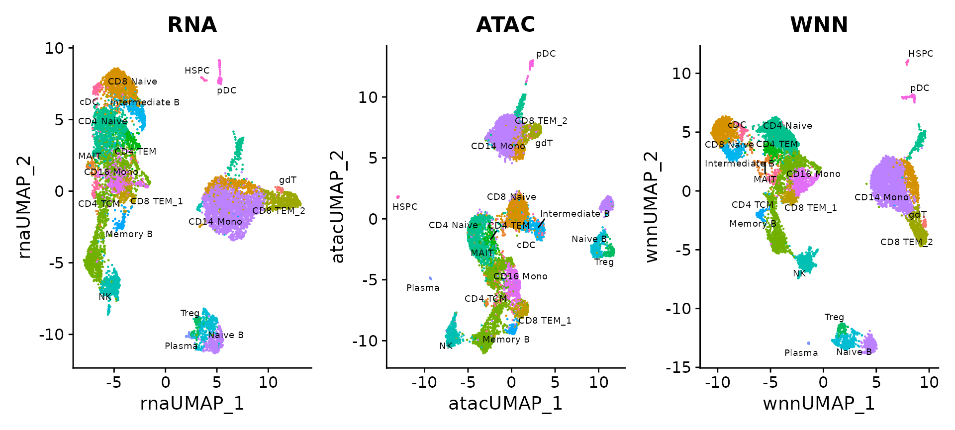
For example, the ATAC-seq data assists in the separation of CD4 and CD8 T cell states. This is due to the presence of multiple loci that exhibit differential accessibility between different T cell subtypes. For example, we can visualize ‘pseudobulk’ tracks of the CD8A locus alongside violin plots of gene expression levels, using tools in the Signac visualization vignette.
## to make the visualization easier, subset T cell clusters
celltype.names <- levels(pbmc)
tcell.names <- grep("CD4|CD8|Treg", celltype.names,value = TRUE)
tcells <- subset(pbmc, idents = tcell.names)
CoveragePlot(tcells, region = 'CD8A', features = 'CD8A', assay = 'ATAC', expression.assay = 'SCT', peaks = FALSE)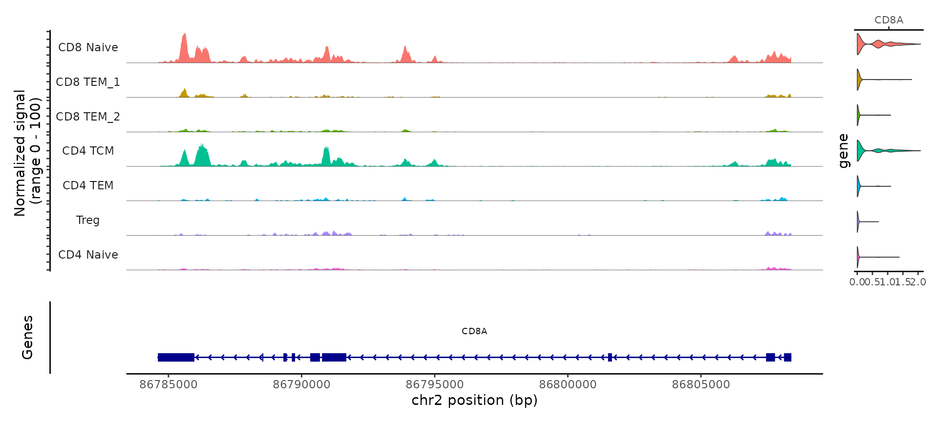
Next, we will examine the accessible regions of each cell to
determine enriched motifs. As described in the Signac
motifs vignette, there are a few ways to do this, but we will use
the chromVAR
package from the Greenleaf lab directly (the RunChromVAR()
wrapper was removed in recent Signac releases). This calculates a
per-cell accessibility score for known motifs, and adds these scores as
a third assay (chromvar) in the Seurat object.
To continue, please make sure you have the following packages installed.
- chromVAR for the analysis of motif accessibility in scATAC-seq
- presto for fast differential expression analyses.
- TFBSTools for TFBS analysis
- JASPAR2020 for JASPAR motif models
- motifmatchr for motif matching
- BSgenome.Hsapiens.UCSC.hg38 for chromVAR
Install command for all dependencies
remotes::install_github("immunogenomics/presto")
BiocManager::install(c("chromVAR", "TFBSTools", "JASPAR2020", "motifmatchr", "BSgenome.Hsapiens.UCSC.hg38"))
library(chromVAR)
library(JASPAR2020)
library(TFBSTools)
library(motifmatchr)
library(BSgenome.Hsapiens.UCSC.hg38)

# Scan the DNA sequence of each peak for the presence of each motif, and create a Motif object
DefaultAssay(pbmc) <- "ATAC"
pwm_set <- getMatrixSet(x = JASPAR2020, opts = list(species = 9606, all_versions = FALSE))
motif.matrix <- CreateMotifMatrix(features = granges(pbmc), pwm = pwm_set, genome = 'hg38', use.counts = FALSE)
motif.object <- CreateMotifObject(data = motif.matrix, pwm = pwm_set)
pbmc <- SetAssayData(pbmc, assay = 'ATAC', layer = 'motifs', new.data = motif.object)

# Build chromVAR input object from ATAC counts
peak_counts <- GetAssayData(pbmc, assay = "ATAC", layer = "counts")
chromvar_input <- SummarizedExperiment::SummarizedExperiment(
  assays = list(counts = peak_counts),
  rowRanges = granges(pbmc)
)
chromvar_input <- chromVAR::addGCBias(chromvar_input, genome = BSgenome.Hsapiens.UCSC.hg38)
motif_ix <- GetMotifData(pbmc, assay = "ATAC", slot = "data")
bg_peaks <- chromVAR::getBackgroundPeaks(chromvar_input)

# Note that this step can take 30-60 minutes
dev <- chromVAR::computeDeviations(
  object = chromvar_input,
  annotations = motif_ix,
  background_peaks = bg_peaks
)
chromvar_scores <- chromVAR::deviationScores(dev)

# Store per-cell motif accessibility as a third assay
pbmc[["chromvar"]] <- CreateAssayObject(counts = chromvar_scores)
pbmc <- SetAssayData(pbmc, assay = "chromvar", layer = "data", new.data = chromvar_scores)
Finally, we explore the multimodal dataset to identify key regulators of each cell state. Paired data provides a unique opportunity to identify transcription factors (TFs) that satisfy multiple criteria, helping to narrow down the list of putative regulators to the most likely candidates. We aim to identify TFs whose expression is enriched in multiple cell types in the RNA measurements, but also have enriched accessibility for their motifs in the ATAC measurements.
As an example and positive control, the CCAAT Enhancer Binding Protein (CEBP) family of proteins, including the TF CEBPB, have been repeatedly shown to play important roles in the differentiation and function of myeloid cells including monocytes and dendritic cells. We can see that both the expression of the CEBPB, and the accessibility of the MA0466.2.4 motif (which encodes the binding site for CEBPB), are both enriched in monocytes.
#returns MA0466.2
motif.name <- ConvertMotifID(pbmc, name = 'CEBPB')
gene_plot <- FeaturePlot(pbmc, features = "sct_CEBPB", reduction = 'wnn.umap')
motif_plot <- FeaturePlot(pbmc, features = motif.name, min.cutoff = 0, cols = c("lightgrey", "darkred"), reduction = 'wnn.umap')
gene_plot | motif_plot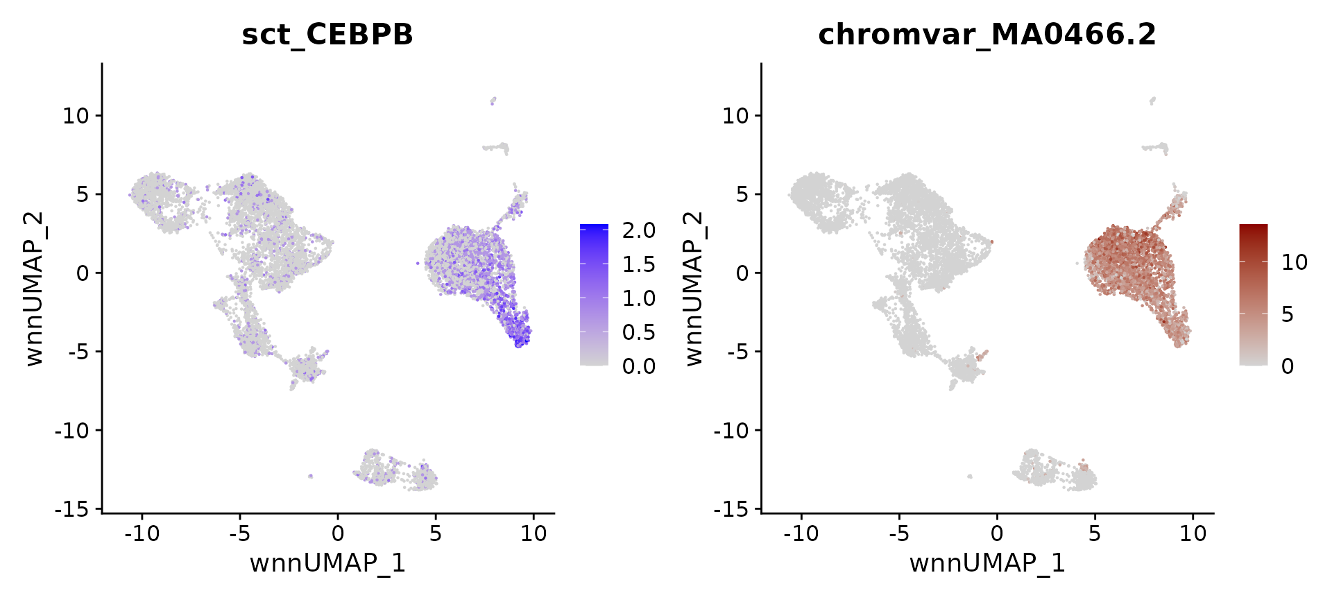
We’d like to quantify this relationship, and search across all cell
types to find similar examples. To do so, we will use the
presto package to perform fast differential expression. We
run two tests: one using gene expression data, and the other using
chromVAR motif accessibilities. presto calculates a p-value
based on the Wilcox rank sum test, which is also the default test in
Seurat, and we restrict our search to TFs that return significant
results in both tests.
presto also calculates an “AUC” statistic, which
reflects the power of each gene (or motif) to serve as a marker of cell
type. A maximum AUC value of 1 indicates a perfect marker. Since the AUC
statistic is on the same scale for both genes and motifs, we take the
average of the AUC values from the two tests, and use this to rank TFs
for each cell type:
markers_rna <- presto:::wilcoxauc.Seurat(X = pbmc, group_by = 'celltype', assay = 'data', seurat_assay = 'SCT')
markers_motifs <- presto:::wilcoxauc.Seurat(X = pbmc, group_by = 'celltype', assay = 'data', seurat_assay = 'chromvar')
motif.names <- markers_motifs$feature
colnames(markers_rna) <- paste0("RNA.", colnames(markers_rna))
colnames(markers_motifs) <- paste0("motif.", colnames(markers_motifs))
markers_rna$gene <- markers_rna$RNA.feature
markers_motifs$gene <- ConvertMotifID(pbmc, id = motif.names)
# a simple function to implement the procedure above
topTFs <- function(celltype, padj.cutoff = 1e-2) {
  ctmarkers_rna <- dplyr::filter(
    markers_rna, RNA.group == celltype, RNA.padj < padj.cutoff, RNA.logFC > 0) %>%
    arrange(-RNA.auc)
  ctmarkers_motif <- dplyr::filter(
    markers_motifs, motif.group == celltype, motif.padj < padj.cutoff, motif.logFC > 0) %>%
    arrange(-motif.auc)
  top_tfs <- inner_join(
    x = ctmarkers_rna[, c(2, 11, 6, 7)],
    y = ctmarkers_motif[, c(2, 1, 11, 6, 7)], by = "gene"
  )
  top_tfs$avg_auc <- (top_tfs$RNA.auc + top_tfs$motif.auc) / 2
  top_tfs <- arrange(top_tfs, -avg_auc)
  return(top_tfs)
}
We can now compute, and visualize, putative regulators for any cell type. We recover well-established regulators, including TBX21 for NK cells, IRF4 for plasma cells, SOX4 for hematopoietic progenitors, EBF1 and PAX5 for B cells, IRF8 and TCF4 for pDC. We believe that similar strategies can be used to help focus on a set of putative regulators in diverse systems.
# identify top markers in NK and visualize
head(topTFs("NK"), 3)
## RNA.group gene RNA.auc RNA.pval motif.group motif.feature motif.auc
## 1 NK TBX21 0.7259435 0.000000e+00 NK MA0690.1 0.9159281
## 2 NK EOMES 0.5891801 2.551087e-99 NK MA0800.1 0.9229104
## 3 NK RUNX3 0.7705084 2.645023e-119 NK MA0684.2 0.6806707
## motif.pval avg_auc
## 1 8.936445e-204 0.8209358
## 2 1.327574e-210 0.7560452
## 3 5.808442e-40 0.7255896
motif.name <- ConvertMotifID(pbmc, name = 'TBX21')
gene_plot <- FeaturePlot(pbmc, features = "sct_TBX21", reduction = 'wnn.umap')
motif_plot <- FeaturePlot(pbmc, features = motif.name, min.cutoff = 0, cols = c("lightgrey", "darkred"), reduction = 'wnn.umap')
gene_plot | motif_plot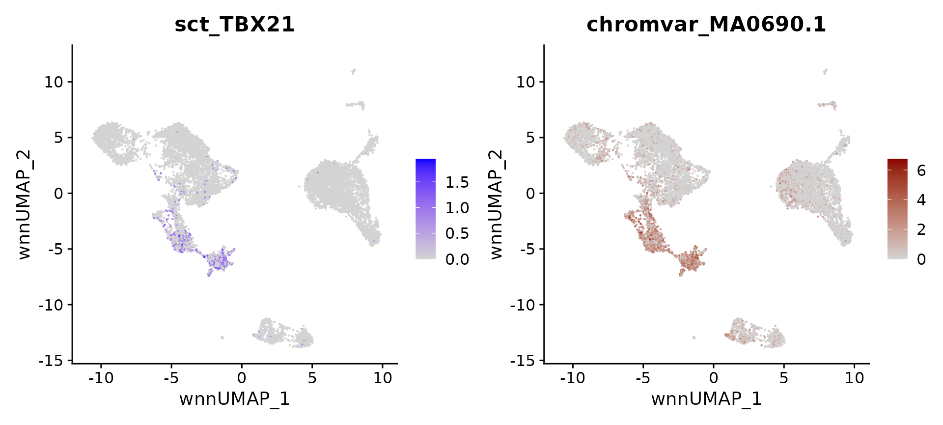
# identify top markers in pDC and visualize
head(topTFs("pDC"), 3)
## RNA.group gene RNA.auc RNA.pval motif.group motif.feature motif.auc
## 1 pDC TCF4 0.9998216 1.229195e-165 pDC MA0830.2 0.9953407
## 2 pDC IRF8 0.9904051 9.643535e-126 pDC MA0652.1 0.8855703
## 3 pDC SPIB 0.9130938 0.000000e+00 pDC MA0081.2 0.9082557
## motif.pval avg_auc
## 1 2.108563e-70 0.9975812
## 2 2.291038e-43 0.9379877
## 3 2.092046e-48 0.9106747
motif.name <- ConvertMotifID(pbmc, name = 'TCF4')
gene_plot <- FeaturePlot(pbmc, features = "sct_TCF4", reduction = 'wnn.umap')
motif_plot <- FeaturePlot(pbmc, features = motif.name, min.cutoff = 0, cols = c("lightgrey", "darkred"), reduction = 'wnn.umap')
gene_plot | motif_plot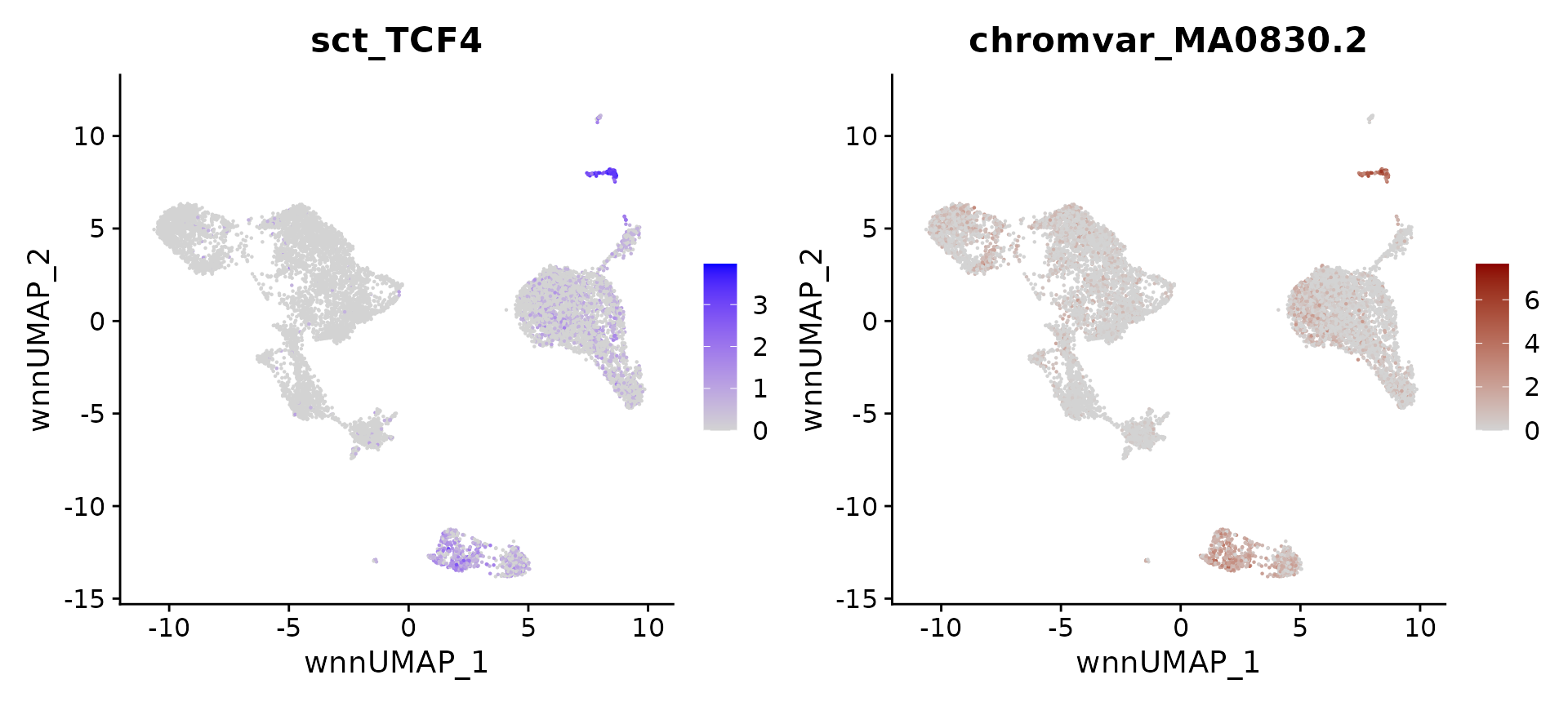
# identify top markers in HSPC and visualize
head(topTFs("CD16 Mono"),3)
## RNA.group gene RNA.auc RNA.pval motif.group motif.feature motif.auc
## 1 CD16 Mono SPI1 0.8807598 3.914255e-298 CD16 Mono MA0080.5 0.8868572
## 2 CD16 Mono CEBPB 0.8653644 4.600997e-289 CD16 Mono MA0466.2 0.7837699
## 3 CD16 Mono MEF2C 0.7136179 1.245914e-79 CD16 Mono MA0497.1 0.8060539
## motif.pval avg_auc
## 1 7.875578e-193 0.8838085
## 2 1.110157e-104 0.8245672
## 3 1.902371e-121 0.7598359
motif.name <- ConvertMotifID(pbmc, name = 'SPI1')
gene_plot <- FeaturePlot(pbmc, features = "sct_SPI1", reduction = 'wnn.umap')
motif_plot <- FeaturePlot(pbmc, features = motif.name, min.cutoff = 0, cols = c("lightgrey", "darkred"), reduction = 'wnn.umap')
gene_plot | motif_plot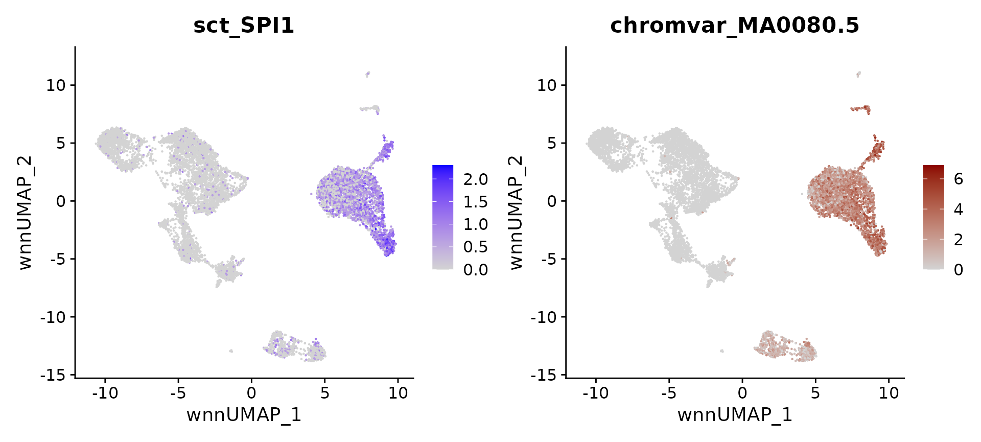
# identify top markers in other cell types
head(topTFs("Naive B"), 3)
## RNA.group gene RNA.auc RNA.pval motif.group motif.feature motif.auc
## 1 Naive B TCF4 0.8421536 2.687809e-245 Naive B MA0830.2 0.9065022
## 2 Naive B EBF1 0.9145448 0.000000e+00 Naive B MA0154.4 0.7566437
## 3 Naive B POU2F2 0.6942501 5.538849e-41 Naive B MA0507.1 0.9734101
## motif.pval avg_auc
## 1 2.886196e-148 0.8743279
## 2 3.020555e-60 0.8355943
## 3 2.332838e-200 0.8338301
head(topTFs("HSPC"), 3)## RNA.group gene RNA.auc RNA.pval motif.group motif.feature motif.auc
## 1 HSPC SOX4 0.9864796 2.339035e-71 HSPC MA0867.2 0.6830497
## 2 HSPC MEIS1 0.8255399 1.754792e-315 HSPC MA0498.2 0.6924225
## 3 HSPC GATA2 0.6730769 0.000000e+00 HSPC MA0036.3 0.8275008
## motif.pval avg_auc
## 1 1.241915e-03 0.8347646
## 2 6.877492e-04 0.7589812
## 3 7.591798e-09 0.7502889
head(topTFs("Plasma"), 3)## RNA.group gene RNA.auc RNA.pval motif.group motif.feature motif.auc
## 1 Plasma IRF4 0.8189848 5.215108e-35 Plasma MA1419.1 0.9776046
## 2 Plasma MEF2C 0.9110384 3.120495e-12 Plasma MA0497.1 0.7596637
## 3 Plasma TCF4 0.8049409 6.810635e-12 Plasma MA0830.2 0.7840848
## motif.pval avg_auc
## 1 2.334627e-12 0.8982947
## 2 1.374353e-04 0.8353511
## 3 3.028306e-05 0.7945129Session Info
## R version 4.5.2 (2025-10-31)
## Platform: x86_64-pc-linux-gnu
## Running under: Ubuntu 24.04.4 LTS
##
## Matrix products: default
## BLAS:   /usr/lib/x86_64-linux-gnu/openblas-pthread/libblas.so.3
## LAPACK: /usr/lib/x86_64-linux-gnu/openblas-pthread/libopenblasp-r0.3.26.so;  LAPACK version 3.12.0
##
## locale:
##  [1] LC_CTYPE=en_US.UTF-8       LC_NUMERIC=C
##  [3] LC_TIME=en_US.UTF-8        LC_COLLATE=en_US.UTF-8
##  [5] LC_MONETARY=en_US.UTF-8    LC_MESSAGES=en_US.UTF-8
##  [7] LC_PAPER=en_US.UTF-8       LC_NAME=C
##  [9] LC_ADDRESS=C               LC_TELEPHONE=C
## [11] LC_MEASUREMENT=en_US.UTF-8 LC_IDENTIFICATION=C
##
## time zone: Etc/UTC
## tzcode source: system (glibc)
##
## attached base packages:
## [1] stats4    stats     graphics  grDevices utils     datasets  methods
## [8] base
##
## other attached packages:
##  [1] BSgenome.Hsapiens.UCSC.hg38_1.4.5 BSgenome_1.78.0
##  [3] rtracklayer_1.70.1                BiocIO_1.20.0
##  [5] Biostrings_2.78.0                 XVector_0.50.0
##  [7] motifmatchr_1.32.0                TFBSTools_1.48.0
##  [9] JASPAR2020_0.99.10                chromVAR_1.32.0
## [11] GenomeInfoDb_1.46.2               EnsDb.Hsapiens.v86_2.99.0
## [13] ensembldb_2.34.0                  AnnotationFilter_1.34.0
## [15] GenomicFeatures_1.62.0            AnnotationDbi_1.72.0
## [17] Biobase_2.70.0                    GenomicRanges_1.62.1
## [19] Seqinfo_1.0.0                     IRanges_2.44.0
## [21] S4Vectors_0.48.1                  BiocGenerics_0.56.0
## [23] generics_0.1.4                    Signac_1.17.1
## [25] ggplot2_4.0.3                     future_1.70.0
## [27] dplyr_1.2.0                       cowplot_1.2.0
## [29] bmcite.SeuratData_0.3.0           SeuratData_0.2.2.9002
## [31] Seurat_5.5.0                      SeuratObject_5.4.0
## [33] sp_2.2-1
##
## loaded via a namespace (and not attached):
##   [1] fs_2.1.0                    ProtGenerics_1.42.0
##   [3] matrixStats_1.5.0           spatstat.sparse_3.1-0
##   [5] bitops_1.0-9                DirichletMultinomial_1.52.0
##   [7] httr_1.4.8                  RColorBrewer_1.1-3
##   [9] tools_4.5.2                 sctransform_0.4.3
##  [11] backports_1.5.0             DT_0.34.0
##  [13] R6_2.6.1                    lazyeval_0.2.3
##  [15] uwot_0.2.4                  withr_3.0.2
##  [17] gridExtra_2.3               progressr_0.19.0
##  [19] cli_3.6.6                   textshaping_1.0.5
##  [21] spatstat.explore_3.8-0      fastDummies_1.7.6
##  [23] labeling_0.4.3              sass_0.4.10
##  [25] S7_0.2.1                    spatstat.data_3.1-9
##  [27] ggridges_0.5.7              pbapply_1.7-4
##  [29] pkgdown_2.2.0               Rsamtools_2.26.0
##  [31] systemfonts_1.3.2           foreign_0.8-90
##  [33] dichromat_2.0-0.1           parallelly_1.47.0
##  [35] rstudioapi_0.18.0           RSQLite_2.4.6
##  [37] gtools_3.9.5                ica_1.0-3
##  [39] spatstat.random_3.4-5       Matrix_1.7-5
##  [41] ggbeeswarm_0.7.3            abind_1.4-8
##  [43] lifecycle_1.0.5             yaml_2.3.12
##  [45] SummarizedExperiment_1.40.0 glmGamPoi_1.22.0
##  [47] SparseArray_1.10.10         Rtsne_0.17
##  [49] grid_4.5.2                  blob_1.3.0
##  [51] promises_1.5.0              pwalign_1.6.0
##  [53] crayon_1.5.3                miniUI_0.1.2
##  [55] lattice_0.22-7              beachmat_2.26.0
##  [57] cigarillo_1.0.0             KEGGREST_1.50.0
##  [59] pillar_1.11.1               knitr_1.51
##  [61] rjson_0.2.23                future.apply_1.20.2
##  [63] codetools_0.2-20            fastmatch_1.1-8
##  [65] glue_1.8.0                  spatstat.univar_3.1-7
##  [67] data.table_1.18.2.1         vctrs_0.7.1
##  [69] png_0.1-9                   spam_2.11-3
##  [71] gtable_0.3.6                cachem_1.1.0
##  [73] xfun_0.56                   S4Arrays_1.10.1
##  [75] mime_0.13                   survival_3.8-3
##  [77] RcppRoll_0.3.2              fitdistrplus_1.2-6
##  [79] ROCR_1.0-12                 nlme_3.1-168
##  [81] bit64_4.6.0-1               RcppAnnoy_0.0.23
##  [83] bslib_0.10.0                irlba_2.3.7
##  [85] vipor_0.4.7                 KernSmooth_2.23-26
##  [87] otel_0.2.0                  rpart_4.1.24
##  [89] seqLogo_1.76.0              colorspace_2.1-2
##  [91] DBI_1.3.0                   Hmisc_5.2-5
##  [93] nnet_7.3-20                 ggrastr_1.0.2
##  [95] tidyselect_1.2.1            bit_4.6.0
##  [97] compiler_4.5.2              curl_7.0.0
##  [99] htmlTable_2.5.0             hdf5r_1.3.12
## [101] desc_1.4.3                  DelayedArray_0.36.1
## [103] plotly_4.12.0               caTools_1.18.3
## [105] checkmate_2.3.4             scales_1.4.0
## [107] lmtest_0.9-40               rappdirs_0.3.4
## [109] nabor_0.5.0                 stringr_1.6.0
## [111] digest_0.6.39               goftest_1.2-3
## [113] presto_1.0.0                spatstat.utils_3.2-2
## [115] rmarkdown_2.30              htmltools_0.5.9
## [117] pkgconfig_2.0.3             base64enc_0.1-6
## [119] sparseMatrixStats_1.22.0    MatrixGenerics_1.22.0
## [121] fastmap_1.2.0               rlang_1.2.0
## [123] htmlwidgets_1.6.4           UCSC.utils_1.6.1
## [125] DelayedMatrixStats_1.32.0   shiny_1.13.0
## [127] farver_2.1.2                jquerylib_0.1.4
## [129] zoo_1.8-15                  jsonlite_2.0.0
## [131] BiocParallel_1.44.0         VariantAnnotation_1.56.0
## [133] RCurl_1.98-1.18             magrittr_2.0.5
## [135] Formula_1.2-5               dotCall64_1.2
## [137] patchwork_1.3.2             Rcpp_1.1.1-1.1
## [139] reticulate_1.46.0           stringi_1.8.7
## [141] MASS_7.3-65                 plyr_1.8.9
## [143] parallel_4.5.2              listenv_0.10.1
## [145] ggrepel_0.9.8               deldir_2.0-4
## [147] splines_4.5.2               tensor_1.5.1
## [149] igraph_2.3.0                spatstat.geom_3.7-3
## [151] RcppHNSW_0.6.0              reshape2_1.4.5
## [153] TFMPvalue_1.0.0             XML_3.99-0.23
## [155] evaluate_1.0.5              biovizBase_1.58.0
## [157] httpuv_1.6.16               RANN_2.6.2
## [159] tidyr_1.3.2                 purrr_1.2.1
## [161] polyclip_1.10-7             scattermore_1.2
## [163] xtable_1.8-8                restfulr_0.0.16
## [165] RSpectra_0.16-2             later_1.4.8
## [167] viridisLite_0.4.3           ragg_1.5.1
## [169] tibble_3.3.1                memoise_2.0.1
## [171] beeswarm_0.4.0              GenomicAlignments_1.46.0
## [173] cluster_2.1.8.2             globals_0.19.1