Using Seurat with multimodal data
Compiled: April 28, 2026
Source:vignettes/multimodal_vignette.Rmd
multimodal_vignette.RmdLoad in the data
The ability to make simultaneous measurements of multiple data types from the same cell, known as multimodal analysis, represents an exciting frontier for single-cell genomics. We have previously highlighted some methods of interest, including CITE-seq, which enables the simultaneous measurements of transcriptomes and cell-surface proteins from the same cell; and the 10x multiome kit, which allows for the paired measurements of cellular transcriptome and chromatin accessibility (i.e scRNA-seq+scATAC-seq). Other modalities that can be measured alongside cellular transcriptomes include genetic perturbations, cellular methylomes, and hashtag oligos (for example, from Cell Hashing). The field has rapidly expanded over the past few years, and we are excited to see the continued development of new technologies for multimodal single-cell analysis.
We have designed Seurat to enable for the seamless storage, analysis, and exploration of diverse multimodal single-cell datasets. We note that Seurat also enables more advanced techniques for the analysis of multimodal data, in particular the application of our Weighted Nearest Neighbors (WNN) approach that enables simultaneous clustering of cells based on a weighted combination of both modalities, and you can explore this functionality here.
Here we present an introductory workflow for creating a multimodal Seurat object and performing an initial analysis. For example, we demonstrate how to cluster a CITE-seq dataset on the basis of the measured cellular transcriptomes, and subsequently discover cell surface proteins that are enriched in each cluster.
In this vignette, we analyze a dataset of 8,617 cord blood mononuclear cells (CBMCs): transcriptomic measurements are paired with abundance estimates for 11 surface proteins, whose levels are quantified with DNA-barcoded antibodies.
First, we load in two count matrices–one for the RNA measurements, and one for the antibody-derived tags (ADT). You can download the ADT file here and the RNA file here.
# Load in the RNA UMI matrix

# Note that this dataset also contains ~5% of mouse cells, which we can use as negative
# controls for the protein measurements For this reason, the gene expression matrix has HUMAN_
# or MOUSE_ appended to the beginning of each gene
cbmc.rna <- as.sparse(read.csv(file = "/brahms/shared/vignette-data/GSE100866_CBMC_8K_13AB_10X-RNA_umi.csv.gz",
    sep = ",", header = TRUE, row.names = 1))

# To make life a bit easier going forward, we're going to discard all but the top 100 most
# highly expressed mouse genes, and remove the 'HUMAN_' from the CITE-seq prefix
cbmc.rna <- CollapseSpeciesExpressionMatrix(cbmc.rna)

# Load in the ADT UMI matrix
cbmc.adt <- as.sparse(read.csv(file = "/brahms/shared/vignette-data/GSE100866_CBMC_8K_13AB_10X-ADT_umi.csv.gz",
    sep = ",", header = TRUE, row.names = 1))

# Note that since measurements were made in the same cells, the two matrices have identical
# column names
all.equal(colnames(cbmc.rna), colnames(cbmc.adt))
## [1] TRUESet up a Seurat object with the RNA and ADT data
We create a Seurat object with the RNA data, and add the ADT data as a second assay:
# creates a Seurat object based on the scRNA-seq data
cbmc <- CreateSeuratObject(counts = cbmc.rna)

# We can see that by default, the cbmc object contains an assay storing RNA measurement
Assays(cbmc)
## [1] "RNA"
# Create a new assay to store ADT information
adt_assay <- CreateAssay5Object(counts = cbmc.adt)

# Add this assay to the previously created Seurat object
cbmc[["ADT"]] <- adt_assay

# Validate that the object now contains multiple assays
Assays(cbmc)
## [1] "RNA" "ADT"
# Extract a list of features measured in the ADT assay
rownames(cbmc[["ADT"]])
## [1] "CD3" "CD4" "CD8" "CD45RA" "CD56" "CD16" "CD10" "CD11c"
## [9] "CD14" "CD19" "CD34" "CCR5" "CCR7"Note that we can easily switch back and forth between the two assays to specify the default for visualization and analysis:
# List the current default assay
DefaultAssay(cbmc)
## [1] "RNA"
# Switch the default to ADT
DefaultAssay(cbmc) <- "ADT"
DefaultAssay(cbmc)
## [1] "ADT"Cluster cells on the basis of their scRNA-seq profiles
The steps below represent a quick clustering of the PBMCs based on the scRNA-seq data. For more detail on individual steps or more advanced options, see our PBMC clustering guided tutorial here
# Note that all operations below are performed on the RNA assay Set and verify that the
# default assay is RNA
DefaultAssay(cbmc) <- "RNA"
DefaultAssay(cbmc)
## [1] "RNA"
# Perform visualization and clustering steps
cbmc <- NormalizeData(cbmc)
cbmc <- FindVariableFeatures(cbmc)
cbmc <- ScaleData(cbmc)
cbmc <- RunPCA(cbmc, verbose = FALSE)
cbmc <- FindNeighbors(cbmc, dims = 1:30)
cbmc <- FindClusters(cbmc, resolution = 0.8, verbose = FALSE)
cbmc <- RunUMAP(cbmc, dims = 1:30)

DimPlot(cbmc, label = TRUE)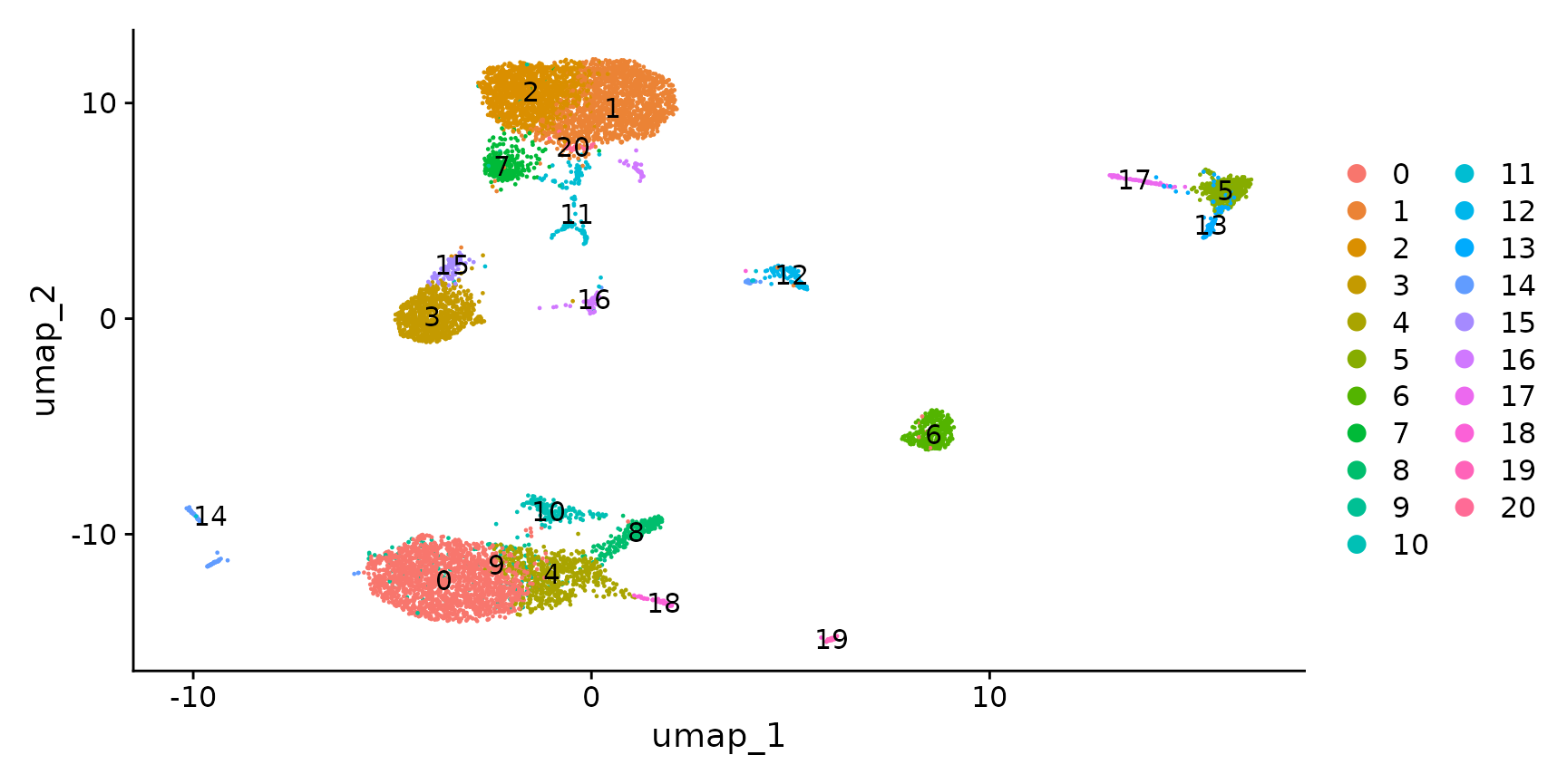
Visualize multiple modalities side-by-side
Now that we have obtained clusters from scRNA-seq profiles, we can visualize the expression of either protein or RNA molecules in our dataset. Importantly, Seurat provides a couple ways to switch between modalities, and specify which modality you are interested in analyzing or visualizing. This is particularly important as, in some cases, the same feature can be present in multiple modalities–for example, this dataset contains independent measurements of the B cell marker CD19 (both protein and RNA levels).
# Normalize ADT data,
DefaultAssay(cbmc) <- "ADT"
cbmc <- NormalizeData(cbmc, normalization.method = "CLR", margin = 2)
DefaultAssay(cbmc) <- "RNA"

# Note that the following command is an alternative but returns the same result
cbmc <- NormalizeData(cbmc, normalization.method = "CLR", margin = 2, assay = "ADT")

# Now, we will visualize CD19 levels for RNA and protein By setting the default assay, we can
# visualize one or the other
DefaultAssay(cbmc) <- "ADT"
p1 <- FeaturePlot(cbmc, "CD19", cols = c("lightgrey", "darkgreen")) + ggtitle("CD19 protein")
DefaultAssay(cbmc) <- "RNA"
p2 <- FeaturePlot(cbmc, "CD19") + ggtitle("CD19 RNA")

# Place plots side-by-side
p1 | p2
# Alternately, we can use specific assay keys to specify a specific modality Identify the key
# for the RNA and protein assays
Key(cbmc[["RNA"]])
## [1] "rna_"
Key(cbmc[["ADT"]])## [1] "adt_"
# Now, we can include the key in the feature name, which overrides the default assay
p1 <- FeaturePlot(cbmc, "adt_CD19", cols = c("lightgrey", "darkgreen")) + ggtitle("CD19 protein")
p2 <- FeaturePlot(cbmc, "rna_CD19") + ggtitle("CD19 RNA")
p1 | p2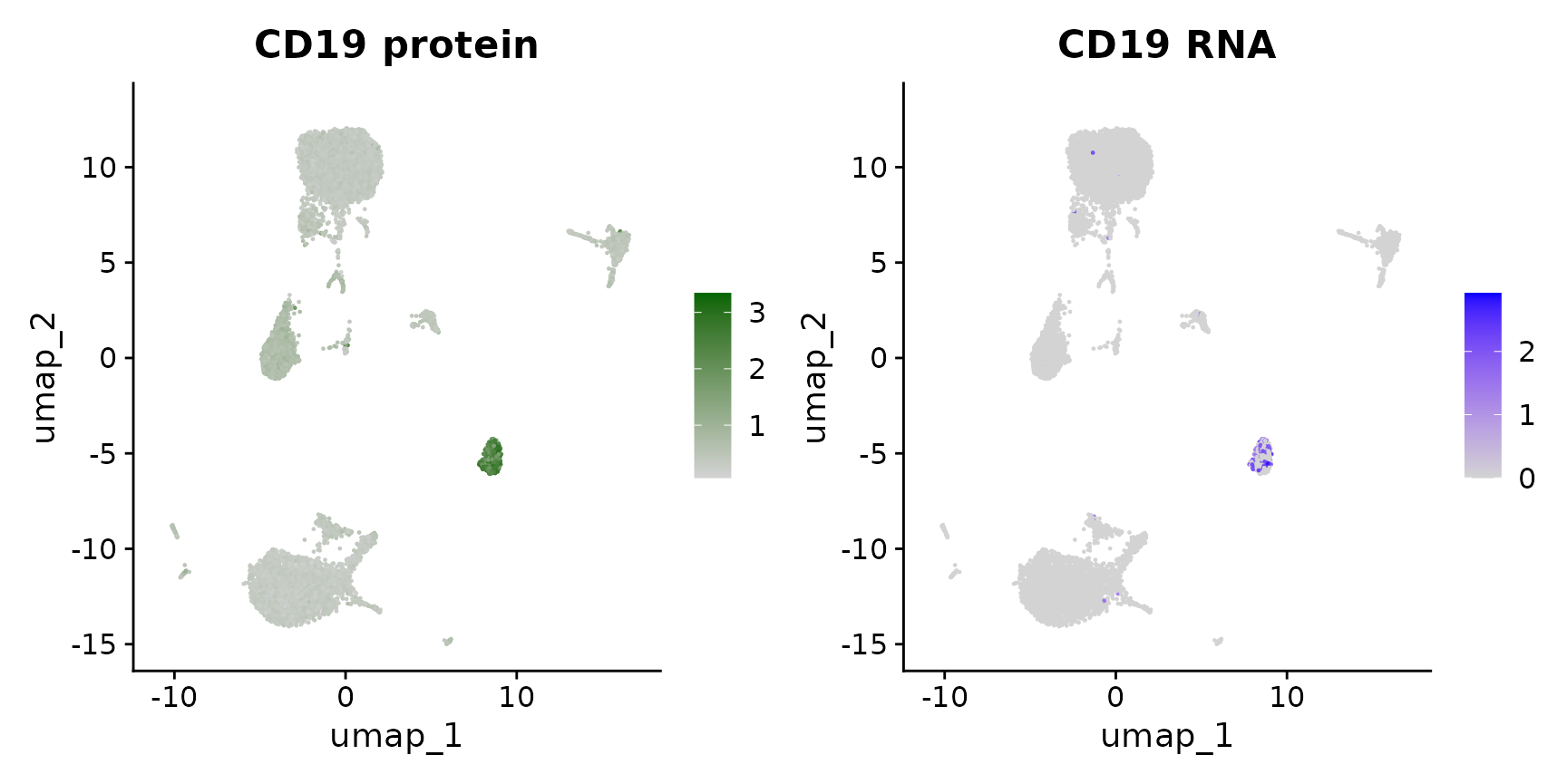
Identify cell surface markers for scRNA-seq clusters
We can leverage our paired CITE-seq measurements to help annotate clusters derived from scRNA-seq, and to identify both protein and RNA markers.
# As we know that CD19 is a B cell marker, we can identify cluster 6 as expressing CD19 on the
# surface
VlnPlot(cbmc, "adt_CD19")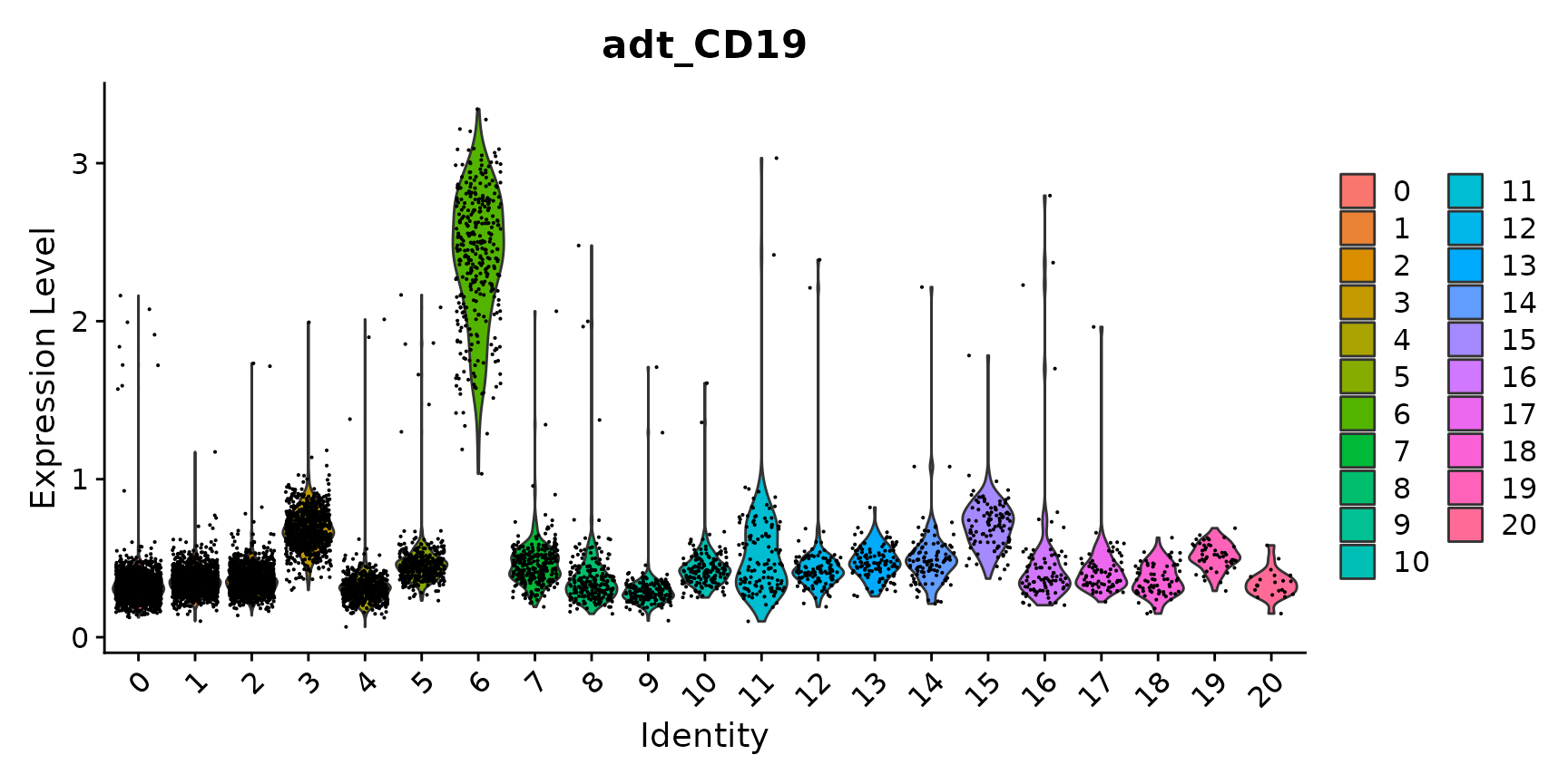
# We can also identify alternative protein and RNA markers for this cluster through
# differential expression
adt_markers <- FindMarkers(cbmc, ident.1 = 6, assay = "ADT")
rna_markers <- FindMarkers(cbmc, ident.1 = 6, assay = "RNA")

head(adt_markers)
## p_val avg_log2FC pct.1 pct.2 p_val_adj
## CD19 2.067533e-215 2.5741873 1 1 2.687793e-214
## CD45RA 8.108073e-109 0.5300346 1 1 1.054049e-107
## CD4 1.123162e-107 -1.6707420 1 1 1.460110e-106
## CD14 7.212876e-106 -1.0332070 1 1 9.376739e-105
## CD3 1.639633e-87 -1.5823056 1 1 2.131523e-86
## CCR5 2.552859e-63 0.3753989 1 1 3.318716e-62
head(rna_markers)## p_val avg_log2FC pct.1 pct.2 p_val_adj
## IGHM 0 6.660187 0.977 0.044 0
## CD79A 0 6.748356 0.965 0.045 0
## TCL1A 0 7.428099 0.904 0.028 0
## CD79B 0 5.525568 0.944 0.089 0
## IGHD 0 7.811884 0.857 0.015 0
## MS4A1 0 7.523215 0.851 0.016 0Additional visualizations of multimodal data
# Draw ADT scatter plots (like biaxial plots for FACS). Note that you can even 'gate' cells if
# desired by using HoverLocator and FeatureLocator
FeatureScatter(cbmc, feature1 = "adt_CD19", feature2 = "adt_CD3")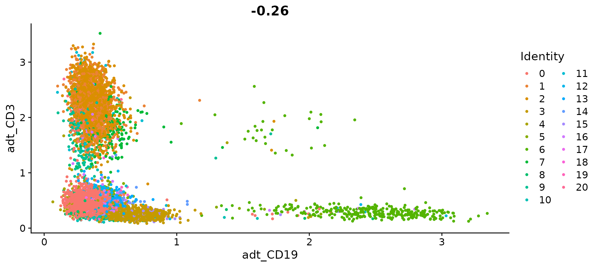
# view relationship between protein and RNA
FeatureScatter(cbmc, feature1 = "adt_CD3", feature2 = "rna_CD3E")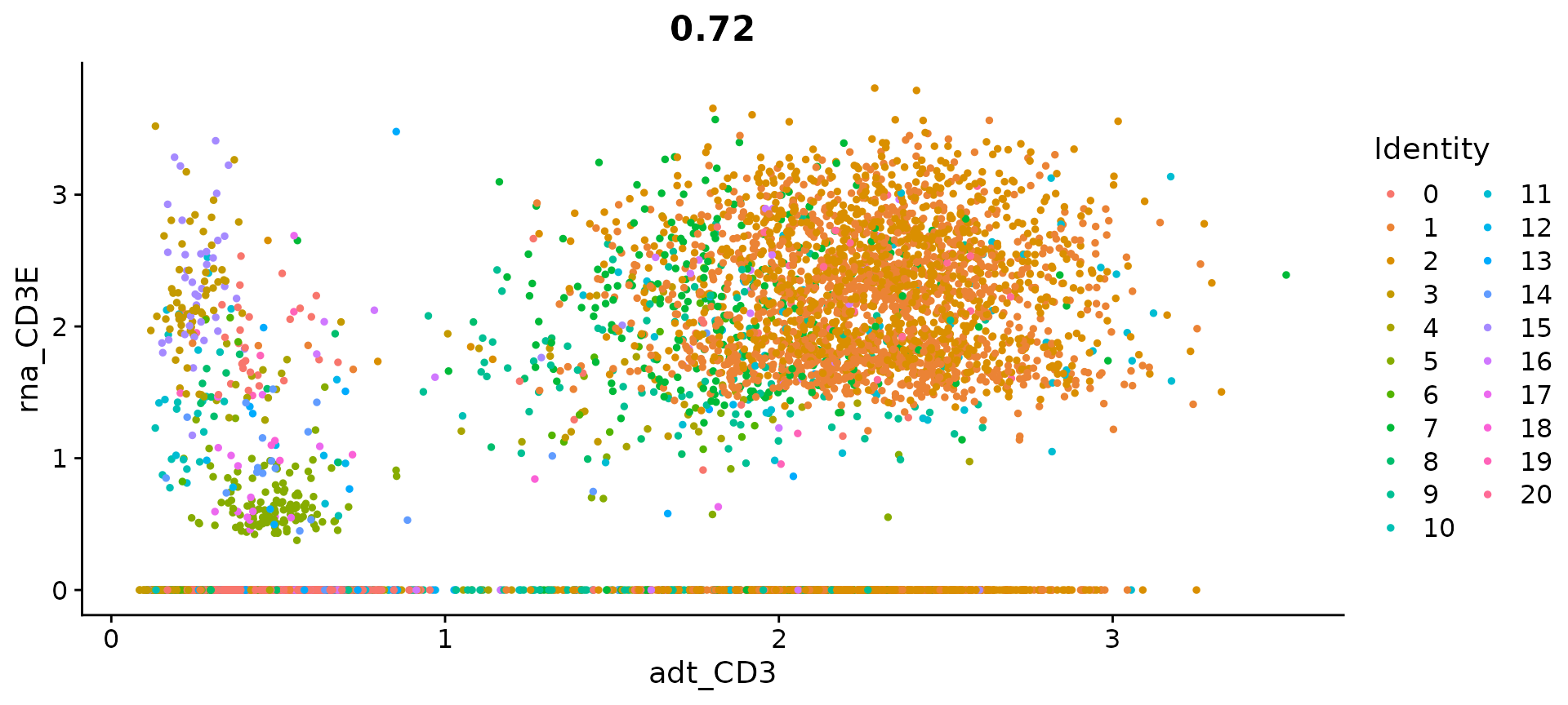
FeatureScatter(cbmc, feature1 = "adt_CD4", feature2 = "adt_CD8")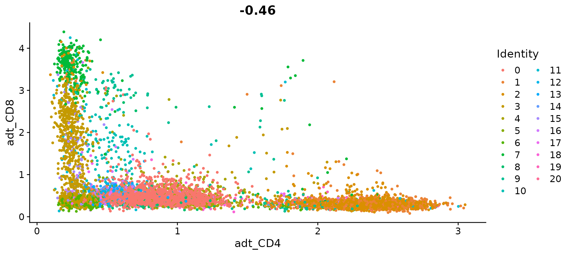
# Let's look at the raw (non-normalized) ADT counts. You can see the values are quite high,
# particularly in comparison to RNA values This is due to the significantly higher protein
# copy number in cells, which significantly reduces 'drop-out' in ADT data
FeatureScatter(cbmc, feature1 = "adt_CD4", feature2 = "adt_CD8", slot = "counts")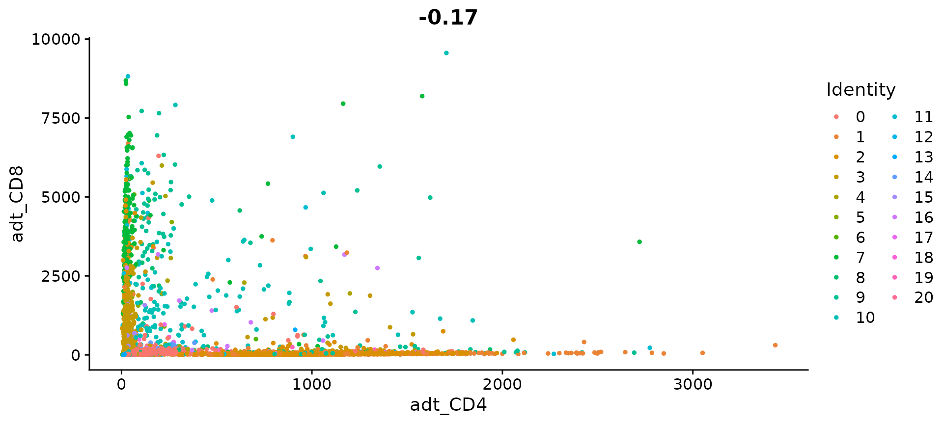
Loading data from 10X multi-modal experiments
Seurat is also able to analyze data from multimodal 10X experiments processed using CellRanger >=v3; as an example, we recreate the plots above using a dataset of 7,900 peripheral blood mononuclear cells (PBMC), freely available from 10X Genomics here.
pbmc10k.data <- Read10X(data.dir = "/brahms/shared/vignette-data/pbmc10k/filtered_feature_bc_matrix/")
rownames(x = pbmc10k.data[["Antibody Capture"]]) <- gsub(pattern = "_[control_]*TotalSeqB", replacement = "",
    x = rownames(x = pbmc10k.data[["Antibody Capture"]]))

pbmc10k <- CreateSeuratObject(counts = pbmc10k.data[["Gene Expression"]], min.cells = 3, min.features = 200)
pbmc10k <- NormalizeData(pbmc10k)
pbmc10k[["ADT"]] <- CreateAssayObject(pbmc10k.data[["Antibody Capture"]][, colnames(x = pbmc10k)])
pbmc10k <- NormalizeData(pbmc10k, assay = "ADT", normalization.method = "CLR")

plot1 <- FeatureScatter(pbmc10k, feature1 = "adt_CD19", feature2 = "adt_CD3", pt.size = 1)
plot2 <- FeatureScatter(pbmc10k, feature1 = "adt_CD4", feature2 = "adt_CD8a", pt.size = 1)
plot3 <- FeatureScatter(pbmc10k, feature1 = "adt_CD3", feature2 = "CD3E", pt.size = 1)
(plot1 + plot2 + plot3) & NoLegend()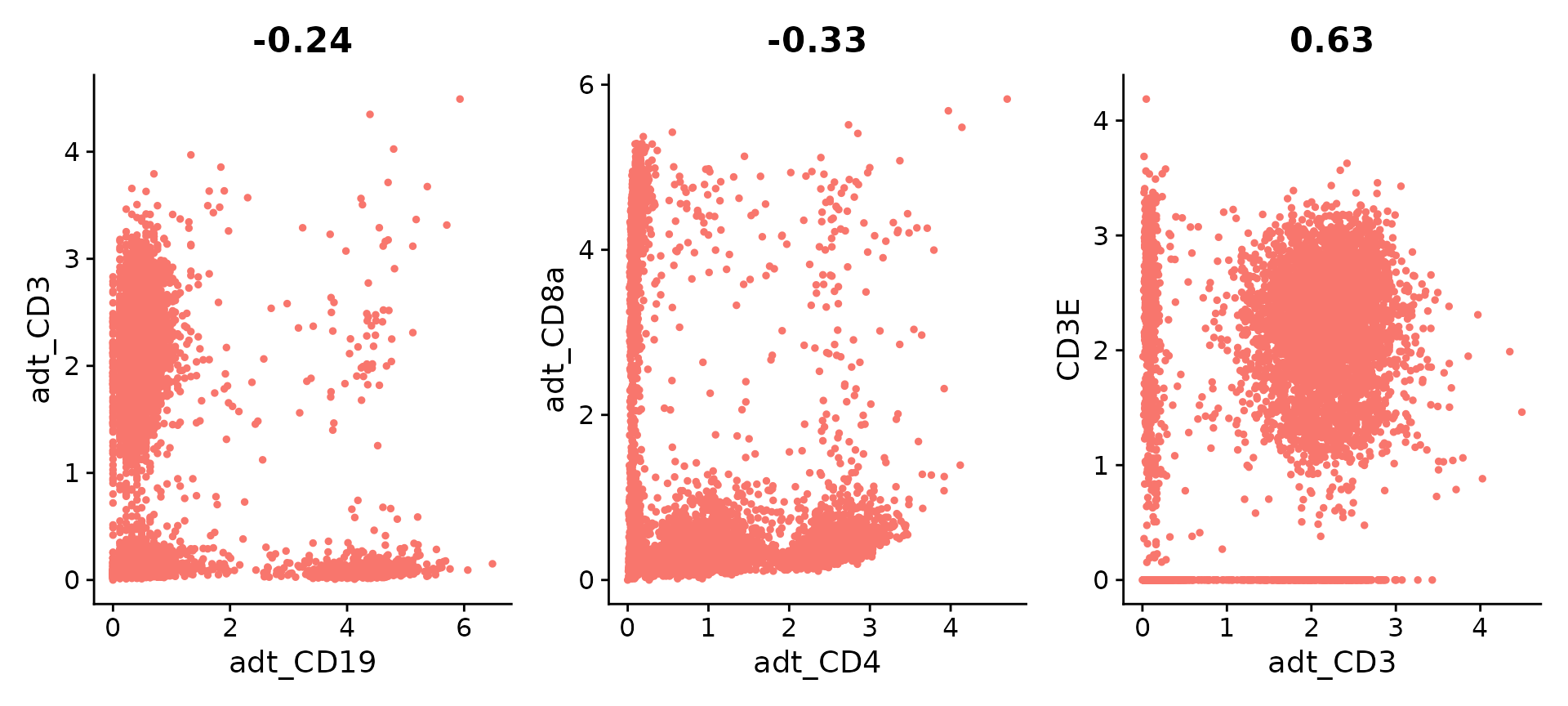
plot <- FeatureScatter(cbmc, feature1 = "adt_CD19", feature2 = "adt_CD3") + NoLegend() + theme(axis.title = element_text(size = 18),
    legend.text = element_text(size = 18))
plot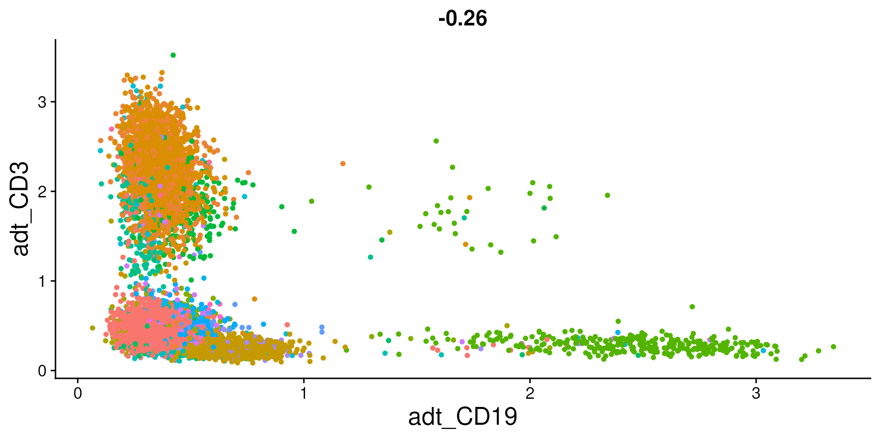
# ggsave(filename = '../output/images/citeseq_plot.jpg', height = 7, width = 12, plot = plot,
# quality = 50)
Additional functionality for multimodal data in Seurat
Seurat also includes additional functionality for the analysis, visualization, and integration of multimodal datasets.
For more information, please explore the resources below:
- Mapping multi-omic datasets across molecular modalities with bridge integration (vignette)
- Defining cellular identity from multimodal data using WNN analysis (vignette)
- Mapping scRNA-seq data onto CITE-seq references (vignette)
- Analyzing spatial transcriptomics data (vignettes)
-
Signac: Analysis, interpretation, and exploration of single-cell chromatin datasets (package) -
Mixscape: an analytical toolkit for pooled single-cell genetic screens (vignette)
Session Info
## R version 4.5.2 (2025-10-31)
## Platform: x86_64-pc-linux-gnu
## Running under: Ubuntu 24.04.4 LTS
##
## Matrix products: default
## BLAS:   /usr/lib/x86_64-linux-gnu/openblas-pthread/libblas.so.3
## LAPACK: /usr/lib/x86_64-linux-gnu/openblas-pthread/libopenblasp-r0.3.26.so;  LAPACK version 3.12.0
##
## locale:
##  [1] LC_CTYPE=en_US.UTF-8       LC_NUMERIC=C
##  [3] LC_TIME=en_US.UTF-8        LC_COLLATE=en_US.UTF-8
##  [5] LC_MONETARY=en_US.UTF-8    LC_MESSAGES=en_US.UTF-8
##  [7] LC_PAPER=en_US.UTF-8       LC_NAME=C
##  [9] LC_ADDRESS=C               LC_TELEPHONE=C
## [11] LC_MEASUREMENT=en_US.UTF-8 LC_IDENTIFICATION=C
##
## time zone: Etc/UTC
## tzcode source: system (glibc)
##
## attached base packages:
## [1] stats     graphics  grDevices utils     datasets  methods   base
##
## other attached packages:
## [1] future_1.70.0      patchwork_1.3.2    ggplot2_4.0.3      Seurat_5.5.0
## [5] SeuratObject_5.4.0 sp_2.2-1
##
## loaded via a namespace (and not attached):
##   [1] RColorBrewer_1.1-3     jsonlite_2.0.0         magrittr_2.0.5
##   [4] spatstat.utils_3.2-2   ggbeeswarm_0.7.3       farver_2.1.2
##   [7] rmarkdown_2.30         fs_2.1.0               ragg_1.5.1
##  [10] vctrs_0.7.1            ROCR_1.0-12            spatstat.explore_3.8-0
##  [13] htmltools_0.5.9        sass_0.4.10            sctransform_0.4.3
##  [16] parallelly_1.47.0      KernSmooth_2.23-26     bslib_0.10.0
##  [19] htmlwidgets_1.6.4      desc_1.4.3             ica_1.0-3
##  [22] plyr_1.8.9             plotly_4.12.0          zoo_1.8-15
##  [25] cachem_1.1.0           igraph_2.3.0           mime_0.13
##  [28] lifecycle_1.0.5        pkgconfig_2.0.3        Matrix_1.7-5
##  [31] R6_2.6.1               fastmap_1.2.0          fitdistrplus_1.2-6
##  [34] shiny_1.13.0           digest_0.6.39          tensor_1.5.1
##  [37] RSpectra_0.16-2        irlba_2.3.7            textshaping_1.0.5
##  [40] labeling_0.4.3         progressr_0.19.0       spatstat.sparse_3.1-0
##  [43] httr_1.4.8             polyclip_1.10-7        abind_1.4-8
##  [46] compiler_4.5.2         withr_3.0.2            S7_0.2.1
##  [49] fastDummies_1.7.6      R.utils_2.13.0         MASS_7.3-65
##  [52] tools_4.5.2            vipor_0.4.7            lmtest_0.9-40
##  [55] otel_0.2.0             beeswarm_0.4.0         httpuv_1.6.16
##  [58] future.apply_1.20.2    goftest_1.2-3          R.oo_1.27.1
##  [61] glue_1.8.0             nlme_3.1-168           promises_1.5.0
##  [64] grid_4.5.2             Rtsne_0.17             cluster_2.1.8.2
##  [67] reshape2_1.4.5         generics_0.1.4         gtable_0.3.6
##  [70] spatstat.data_3.1-9    R.methodsS3_1.8.2      tidyr_1.3.2
##  [73] data.table_1.18.2.1    spatstat.geom_3.7-3    RcppAnnoy_0.0.23
##  [76] ggrepel_0.9.8          RANN_2.6.2             pillar_1.11.1
##  [79] stringr_1.6.0          limma_3.66.0           spam_2.11-3
##  [82] RcppHNSW_0.6.0         later_1.4.8            splines_4.5.2
##  [85] dplyr_1.2.0            lattice_0.22-7         survival_3.8-3
##  [88] deldir_2.0-4           tidyselect_1.2.1       miniUI_0.1.2
##  [91] pbapply_1.7-4          knitr_1.51             gridExtra_2.3
##  [94] scattermore_1.2        xfun_0.56              statmod_1.5.1
##  [97] matrixStats_1.5.0      stringi_1.8.7          lazyeval_0.2.3
## [100] yaml_2.3.12            evaluate_1.0.5         codetools_0.2-20
## [103] tibble_3.3.1           cli_3.6.6              uwot_0.2.4
## [106] xtable_1.8-8           reticulate_1.46.0      systemfonts_1.3.2
## [109] jquerylib_0.1.4        Rcpp_1.1.1-1.1         globals_0.19.1
## [112] spatstat.random_3.4-5  png_0.1-9              ggrastr_1.0.2
## [115] spatstat.univar_3.1-7  parallel_4.5.2         pkgdown_2.2.0
## [118] presto_1.0.0           dotCall64_1.2          listenv_0.10.1
## [121] viridisLite_0.4.3      scales_1.4.0           ggridges_0.5.7
## [124] purrr_1.2.1            rlang_1.2.0            cowplot_1.2.0
## [127] formatR_1.14