Multimodal reference mapping
Compiled: October 31, 2023
Source:vignettes/multimodal_reference_mapping.Rmd
multimodal_reference_mapping.RmdIntro: Seurat v4 Reference Mapping
This vignette introduces the process of mapping query datasets to annotated references in Seurat. In this example, we map one of the first scRNA-seq datasets released by 10X Genomics of 2,700 PBMC to our recently described CITE-seq reference of 162,000 PBMC measured with 228 antibodies. We chose this example to demonstrate how supervised analysis guided by a reference dataset can help to enumerate cell states that would be challenging to find with unsupervised analysis. In a second example, we demonstrate how to serially map Human Cell Atlas datasets of human BMNC profiled from different individuals onto a consistent reference.
We have previously demonstrated how to use reference-mapping approach to annotate cell labels in a query dataset . In Seurat v4, we have substantially improved the speed and memory requirements for integrative tasks including reference mapping, and also include new functionality to project query cells onto a previously computed UMAP visualization.
In this vignette, we demonstrate how to use a previously established reference to interpret an scRNA-seq query:
- Annotate each query cell based on a set of reference-defined cell states
- Project each query cell onto a previously computed UMAP visualization
- Impute the predicted levels of surface proteins that were measured in the CITE-seq reference
To run this vignette please install Seurat v4, available on CRAN. Additionally, you will need to install the SeuratDisk package.
options(SeuratData.repo.use = "http://seurat.nygenome.org")Example 1: Mapping human peripheral blood cells
A Multimodal PBMC Reference Dataset
We load the reference from our recent paper, and visualize the pre-computed UMAP.
reference <- readRDS("/brahms/hartmana/vignette_data/pbmc_multimodal_2023.rds")
DimPlot(object = reference, reduction = "wnn.umap", group.by = "celltype.l2", label = TRUE, label.size = 3, repel = TRUE) + NoLegend()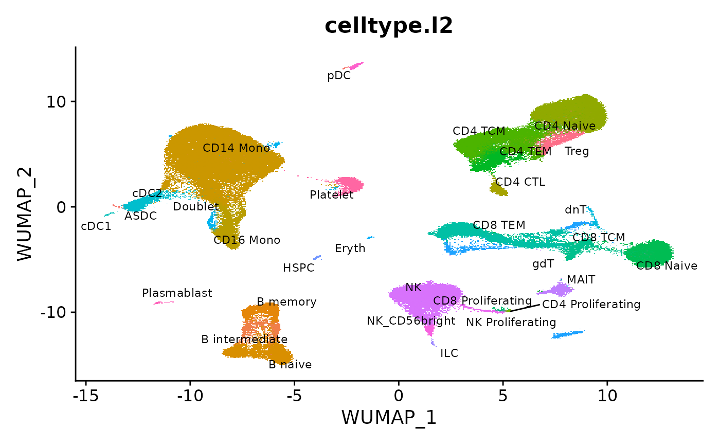
Mapping
To demonstrate mapping to this multimodal reference, we will use a dataset of 2,700 PBMCs generated by 10x Genomics and available via SeuratData.
library(SeuratData)
InstallData('pbmc3k')

pbmc3k <- LoadData('pbmc3k')
pbmc3k <- UpdateSeuratObject(pbmc3k)
The reference was normalized using SCTransform(), so we use the same approach to normalize the query here.
pbmc3k <- SCTransform(pbmc3k, verbose = FALSE)We then find anchors between reference and query. As described in the manuscript, we used a precomputed supervised PCA (spca) transformation for this example. We recommend the use of supervised PCA for CITE-seq datasets, and demonstrate how to compute this transformation on the next tab of this vignette. However, you can also use a standard PCA transformation.
anchors <- FindTransferAnchors(
  reference = reference,
  query = pbmc3k,
  normalization.method = "SCT",
  reference.reduction = "spca",
  dims = 1:50
)
We then transfer cell type labels and protein data from the reference to the query. Additionally, we project the query data onto the UMAP structure of the reference.
pbmc3k <- MapQuery(
  anchorset = anchors,
  query = pbmc3k,
  reference = reference,
  refdata = list(
    celltype.l1 = "celltype.l1",
    celltype.l2 = "celltype.l2",
    predicted_ADT = "ADT"
  ),
  reference.reduction = "spca",
  reduction.model = "wnn.umap"
)
What is
MapQuery doing?
MapQuery() is a wrapper around three functions: TransferData(), IntegrateEmbeddings(), and ProjectUMAP(). TransferData() is used to transfer cell type labels and impute the ADT values. IntegrateEmbeddings() and ProjectUMAP() are used to project the query data onto the UMAP structure of the reference. The equivalent code for doing this with the intermediate functions is below:
pbmc3k <- TransferData(
  anchorset = anchors,
  reference = reference,
  query = pbmc3k,
  refdata = list(
    celltype.l1 = "celltype.l1",
    celltype.l2 = "celltype.l2",
    predicted_ADT = "ADT")
)
pbmc3k <- IntegrateEmbeddings(
  anchorset = anchors,
  reference = reference,
  query = pbmc3k,
  new.reduction.name = "ref.spca"
)
pbmc3k <- ProjectUMAP(
  query = pbmc3k,
  query.reduction = "ref.spca",
  reference = reference,
  reference.reduction = "spca",
  reduction.model = "wnn.umap"
)
Explore the mapping results
We can now visualize the 2,700 query cells. They have been projected into a UMAP visualization defined by the reference, and each has received annotations at two levels of granularity (level 1, and level 2).
p1 = DimPlot(pbmc3k, reduction = "ref.umap", group.by = "predicted.celltype.l1", label = TRUE, label.size = 3, repel = TRUE) + NoLegend()
p2 = DimPlot(pbmc3k, reduction = "ref.umap", group.by = "predicted.celltype.l2", label = TRUE, label.size = 3 ,repel = TRUE) + NoLegend()
p1 + p2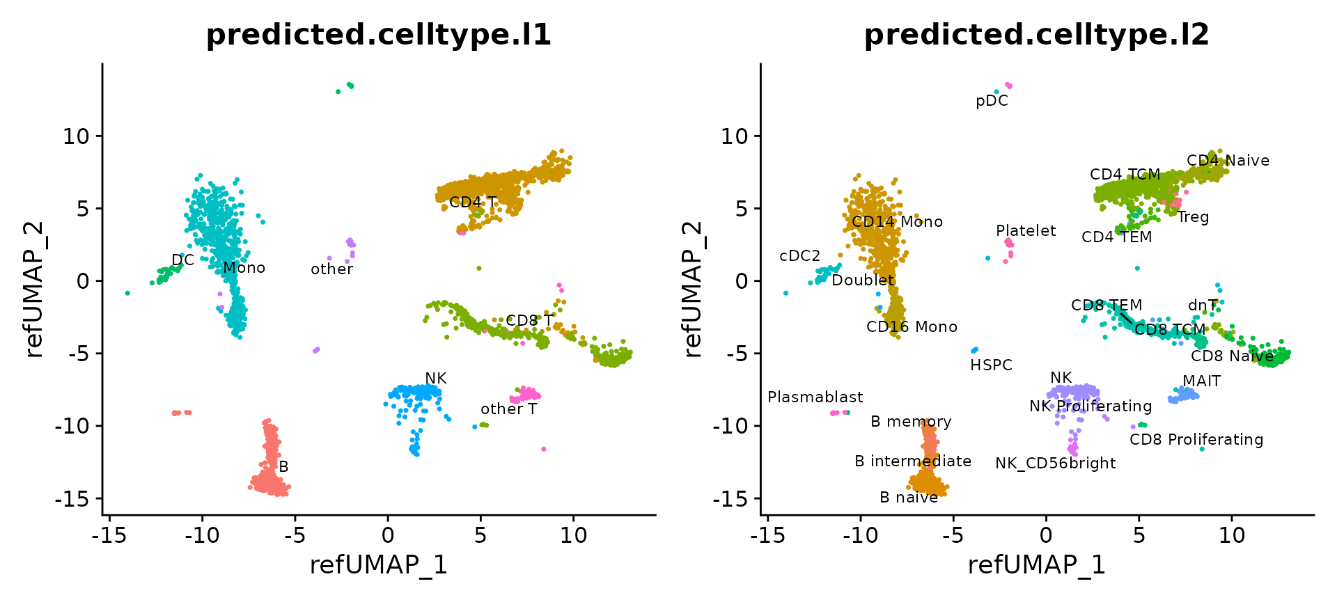
The reference-mapped dataset helps us identify cell types that were previously blended in an unsupervised analysis of the query dataset. Just a few examples include plasmacytoid dendritic cells (pDC), hematopoietic stem and progenitor cells (HSPC), regulatory T cells (Treg), CD8 Naive T cells, cells, CD56+ NK cells, memory, and naive B cells, and plasmablasts.
Each prediction is assigned a score between 0 and 1.
FeaturePlot(pbmc3k, features = c("pDC", "CD16 Mono", "Treg"), reduction = "ref.umap", cols = c("lightgrey", "darkred"), ncol = 3) & theme(plot.title = element_text(size = 10))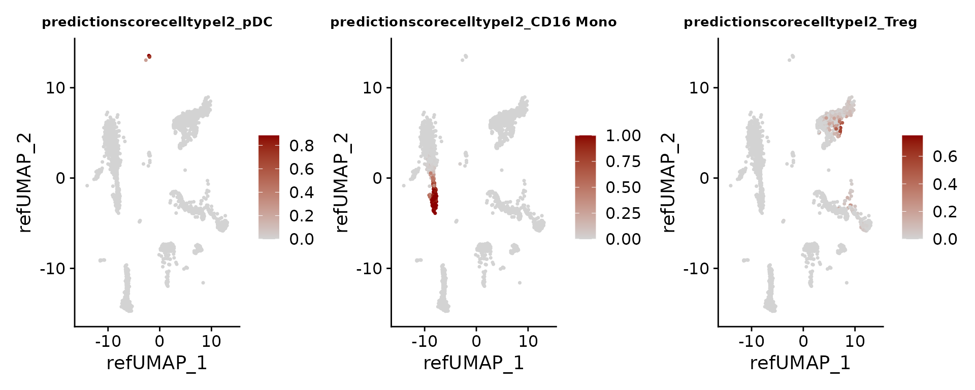
library(ggplot2)
plot <- FeaturePlot(pbmc3k, features = "CD16 Mono",  reduction = "ref.umap", cols = c("lightgrey", "darkred"))  + ggtitle("CD16 Mono") + theme(plot.title = element_text(hjust = 0.5, size = 30)) + labs(color = "Prediction Score") +  xlab("UMAP 1") + ylab("UMAP 2") +
  theme(axis.title = element_text(size = 18), legend.text = element_text(size = 18), legend.title = element_text(size = 25))
ggsave(filename = "../output/images/multimodal_reference_mapping.jpg", height = 7, width = 12, plot = plot, quality = 50)
We can verify our predictions by exploring the expression of canonical marker genes. For example, CLEC4C and LIRA4 have been reported as markers of pDC identity, consistent with our predictions. Similarly, if we perform differential expression to identify markers of Tregs, we identify a set of canonical markers including RTKN2, CTLA4, FOXP3, and IL2RA.
Idents(pbmc3k) <- 'predicted.celltype.l2'
VlnPlot(pbmc3k, features = c("CLEC4C", "LILRA4"), sort = TRUE) + NoLegend()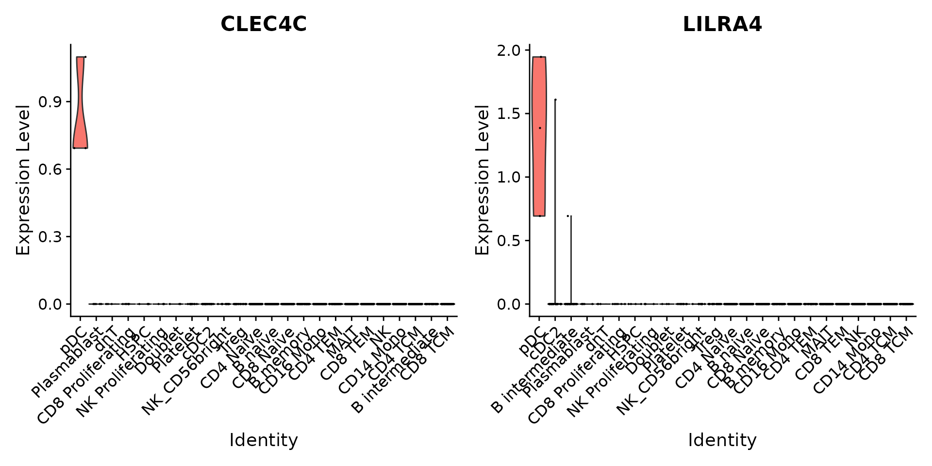
treg_markers <- FindMarkers(pbmc3k, ident.1 = "Treg", only.pos = TRUE, logfc.threshold = 0.1)
print(head(treg_markers))
## p_val avg_log2FC pct.1 pct.2 p_val_adj
## AC004854.4 4.795409e-26 7.800900 0.042 0.000 6.028789e-22
## RP11-297N6.4 4.795409e-26 7.800900 0.042 0.000 6.028789e-22
## RTKN2 4.795409e-26 7.800900 0.042 0.000 6.028789e-22
## CTD-2020K17.4 4.795409e-26 7.800900 0.042 0.000 6.028789e-22
## RP11-1399P15.1 2.782841e-18 4.172869 0.292 0.021 3.498588e-14
## IL2RA 1.808612e-14 4.137935 0.208 0.014 2.273787e-10Finally, we can visualize the imputed levels of surface protein, which were inferred based on the CITE-seq reference.
DefaultAssay(pbmc3k) <- 'predicted_ADT'
# see a list of proteins: rownames(pbmc3k)
FeaturePlot(pbmc3k, features = c("CD3-1", "CD45RA", "IgD"), reduction = "ref.umap", cols = c("lightgrey", "darkgreen"), ncol = 3)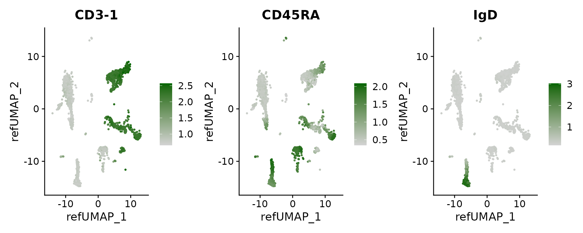
Computing a new UMAP visualiztion
In the previous examples, we visualize the query cells after mapping to the reference-derived UMAP. Keeping a consistent visualization can assist with the interpretation of new datasets. However, if there are cell states that are present in the query dataset that are not represented in the reference, they will project to the most similar cell in the reference. This is the expected behavior and functionality as established by the UMAP package, but can potentially mask the presence of new cell types in the query which may be of interest.
In our manuscript, we map a query dataset containing developing and differentiated neutrophils, which are not included in our reference. We find that computing a new UMAP (‘de novo visualization’) after merging the reference and query can help to identify these populations, as demonstrated in Supplementary Figure 8. In the ‘de novo’ visualization, unique cell states in the query remain separated. In this example, the 2,700 PBMC does not contain unique cell states, but we demonstrate how to compute this visualization below.
We emphasize that if users are attempting to map datasets where the underlying samples are not PBMC, or contain cell types that are not present in the reference, computing a ‘de novo’ visualization is an important step in interpreting their dataset.
reference <- DietSeurat(reference, counts = FALSE, dimreducs = "spca")
pbmc3k <- DietSeurat(pbmc3k, counts = FALSE, dimreducs = "ref.spca")
#merge reference and query
reference$id <- 'reference'
pbmc3k$id <- 'query'
refquery <- merge(reference, pbmc3k)
refquery[["spca"]] <- merge(reference[["spca"]], pbmc3k[["ref.spca"]])
refquery <- RunUMAP(refquery, reduction = 'spca', dims = 1:50)
DimPlot(refquery, group.by = 'id', shuffle = TRUE)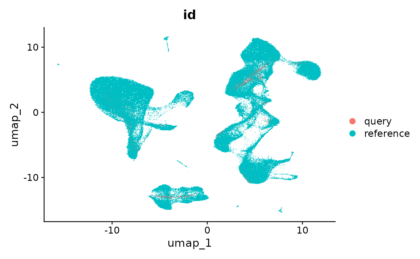
Example 2: Mapping human bone marrow cells
A Multimodal BMNC Reference Dataset
As a second example, we map a dataset of human bone marrow mononuclear (BMNC) cells from eight individual donors, produced by the Human Cell Atlas. As a reference, we use the CITE-seq reference of human BMNC that we analyzed using weighted-nearest neighbor analysis (WNN).
This vignette exhibits the same reference-mapping functionality as the PBMC example on the previous tab. In addition, we also demonstrate:
- How to construct a supervised PCA (sPCA) transformation
- How to serially map multiple datasets to the same reference
- Optimization steps to further enhance to speed of mapping
# Both datasets are available through SeuratData
library(SeuratData)
#load reference data
InstallData("bmcite")
bm <- LoadData(ds = "bmcite")
#load query data
InstallData('hcabm40k')
hcabm40k <- LoadData(ds = "hcabm40k")
The reference dataset contains a WNN graph, reflecting a weighted combination of the RNA and protein data in this CITE-seq experiment.
We can compute a UMAP visualization based on this graph. We set return.model = TRUE, which will enable us to project query datasets onto this visualization.
bm <- RunUMAP(bm, nn.name = "weighted.nn", reduction.name = "wnn.umap",
              reduction.key = "wnnUMAP_", return.model = TRUE)
DimPlot(bm, group.by = "celltype.l2", reduction = "wnn.umap") 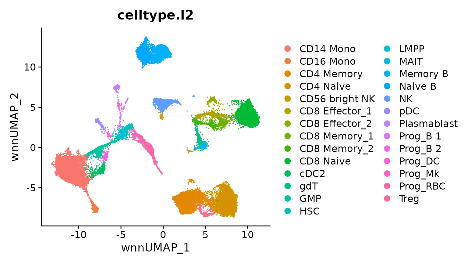
Computing an sPCA transformation
As described in our manuscript, we first compute a ‘supervised’ PCA. This identifies the transformation of the transcriptome data that best encapsulates the structure of the WNN graph. This allows a weighted combination of the protein and RNA measurements to ‘supervise’ the PCA, and highlight the most relevant sources of variation. After computing this transformation, we can project it onto a query dataset. We can also compute and project a PCA projection, but recommend the use of sPCA when working with multimodal references that have been constructed with WNN analysis.
The sPCA calculation is performed once, and then can be rapidly projected onto each query dataset.
Computing a cached neighbor index
Since we will be mapping multiple query samples to the same reference, we can cache particular steps that only involve the reference. This step is optional but will improve speed when mapping multiple samples.
We compute the first 50 neighbors in the sPCA space of the reference. We store this information in the spca.annoy.neighbors object within the reference Seurat object and also cache the annoy index data structure (via cache.index = TRUE).
bm <- FindNeighbors(
  object = bm,
  reduction = "spca",
  dims = 1:50,
  graph.name = "spca.annoy.neighbors",
  k.param = 50,
  cache.index = TRUE,
  return.neighbor = TRUE,
  l2.norm = TRUE
)
How can I save and load a cached annoy index?
If you want to save and load a cached index for a Neighbor object generated with method = "annoy" and cache.index = TRUE, use the SaveAnnoyIndex()/LoadAnnoyIndex() functions. Importantly, this index cannot be saved normally to an RDS or RDA file, so it will not persist correctly across R session restarts or saveRDS/readRDS for the Seurat object containing it. Instead, use LoadAnnoyIndex() to add the Annoy index to the Neighbor object every time R restarts or you load the reference Seurat object from RDS. The file created by SaveAnnoyIndex() can be distributed along with a reference Seurat object, and added to the Neighbor object in the reference.
bm[["spca.annoy.neighbors"]]## A Neighbor object containing the 50 nearest neighbors for 30672 cells
SaveAnnoyIndex(object = bm[["spca.annoy.neighbors"]], file = "/brahms/shared/vignette-data/reftmp.idx")
bm[["spca.annoy.neighbors"]] <- LoadAnnoyIndex(object = bm[["spca.annoy.neighbors"]], file = "/brahms/shared/vignette-data/reftmp.idx")
Query dataset preprocessing
Here we will demonstrate mapping multiple donor bone marrow samples to the multimodal bone marrow reference. These query datasets are derived from the Human Cell Atlas (HCA) Immune Cell Atlas Bone marrow dataset and are available through SeuratData. This dataset is provided as a single merged object with 8 donors. We first split the data back into 8 separate Seurat objects, one for each original donor to map individually.
library(dplyr)
library(SeuratData)
InstallData('hcabm40k')
hcabm40k.batches <- SplitObject(hcabm40k, split.by = "orig.ident")
We then normalize the query in the same manner as the reference. Here, the reference was normalized using log-normalization via NormalizeData(). If the reference had been normalized using SCTransform(), the query must be normalized with SCTransform() as well.
hcabm40k.batches <- lapply(X = hcabm40k.batches, FUN = NormalizeData, verbose = FALSE)Mapping
We then find anchors between each donor query dataset and the multimodal reference. This command is optimized to minimize mapping time, by passing in a pre-computed set of reference neighbors, and turning off anchor filtration.
anchors <- list()
for (i in 1:length(hcabm40k.batches)) {
  anchors[[i]] <- FindTransferAnchors(
    reference = bm,
    query = hcabm40k.batches[[i]],
    k.filter = NA,
    reference.reduction = "spca",
    reference.neighbors = "spca.annoy.neighbors",
    dims = 1:50
  )
}
We then individually map each of the datasets.
Explore the mapping results
Now that mapping is complete, we can visualize the results for individual objects
p1 <- DimPlot(hcabm40k.batches[[1]], reduction = 'ref.umap', group.by = 'predicted.celltype', label.size = 3)
p2 <- DimPlot(hcabm40k.batches[[2]], reduction = 'ref.umap', group.by = 'predicted.celltype', label.size = 3)
p1 + p2 + plot_layout(guides = "collect")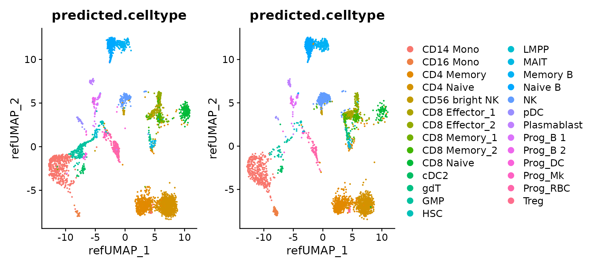
We can also merge all the objects into one dataset. Note that they have all been integrated into a common space, defined by the reference. We can then visualize the results together.
# Merge the batches
hcabm40k <- merge(hcabm40k.batches[[1]], hcabm40k.batches[2:length(hcabm40k.batches)], merge.dr = "ref.umap")
DimPlot(hcabm40k, reduction = "ref.umap", group.by =  "predicted.celltype", label = TRUE, repel = TRUE, label.size = 3) + NoLegend()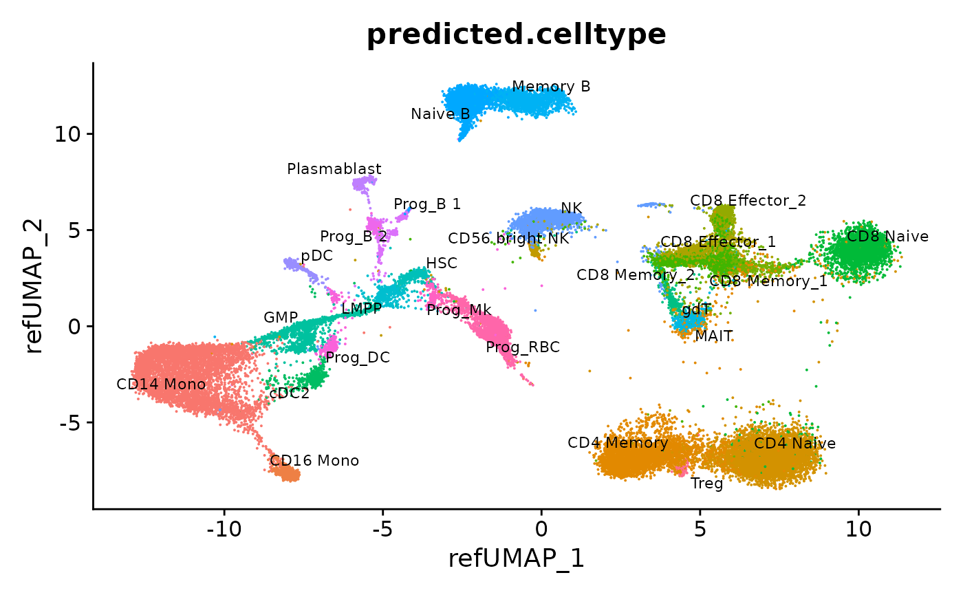
We can visualize gene expression, cluster prediction scores, and (imputed) surface protein levels in the query cells:
p3 <- FeaturePlot(hcabm40k, features = c("rna_TRDC", "rna_MPO", "rna_AVP"), reduction = 'ref.umap',
                  max.cutoff = 3, ncol = 3)

# cell type prediction scores
DefaultAssay(hcabm40k) <- 'prediction.score.celltype'
p4 <- FeaturePlot(hcabm40k, features = c("CD16 Mono", "HSC", "Prog-RBC"), ncol = 3,
                  cols = c("lightgrey", "darkred"))

# imputed protein levels
DefaultAssay(hcabm40k) <- 'predicted_ADT'
p5 <- FeaturePlot(hcabm40k, features = c("CD45RA", "CD16", "CD161"), reduction = 'ref.umap',
                  min.cutoff = 'q10', max.cutoff = 'q99', cols = c("lightgrey", "darkgreen") ,
                  ncol = 3)
p3 / p4 / p5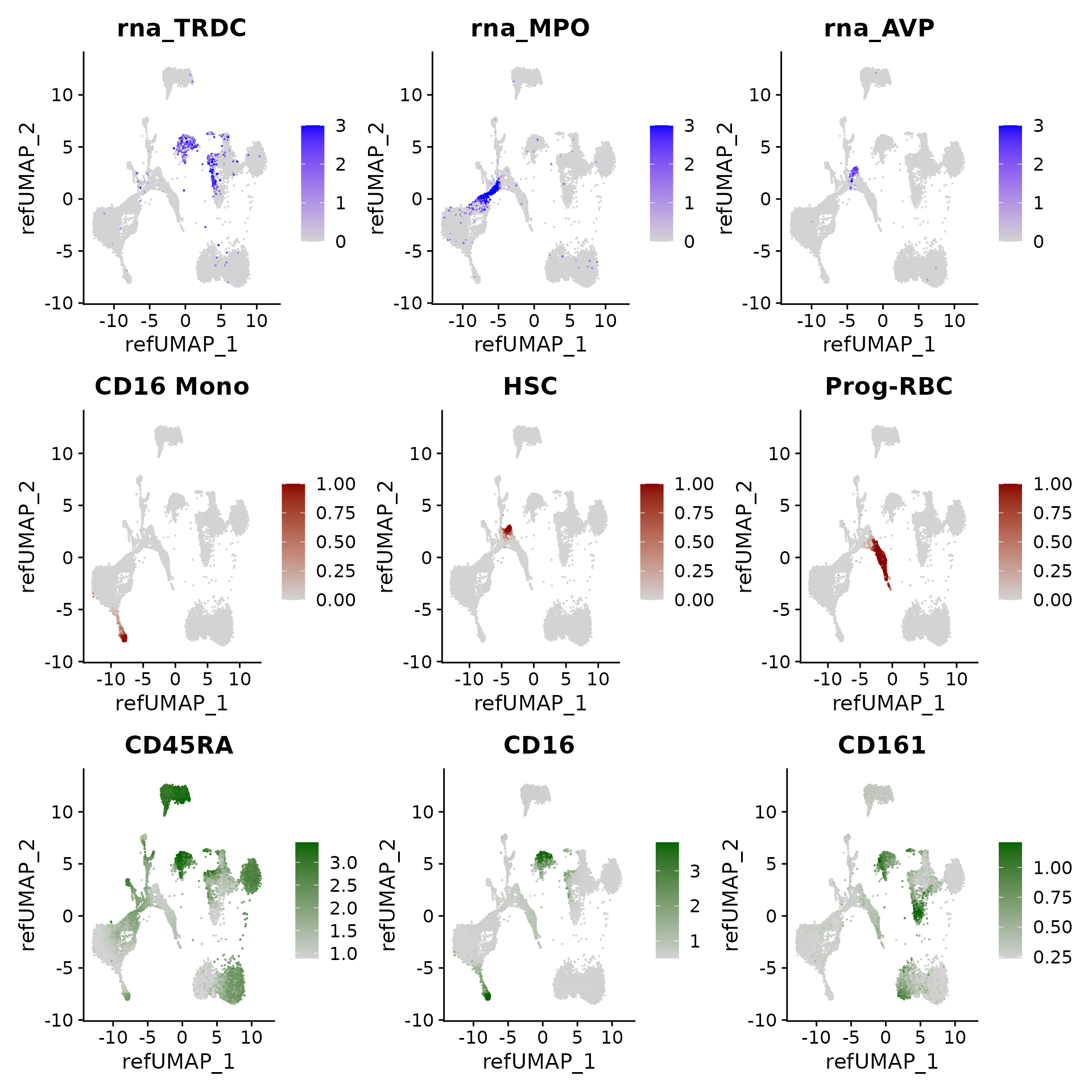
Session Info
## R version 4.2.2 Patched (2022-11-10 r83330)
## Platform: x86_64-pc-linux-gnu (64-bit)
## Running under: Ubuntu 20.04.6 LTS
##
## Matrix products: default
## BLAS:   /usr/lib/x86_64-linux-gnu/blas/libblas.so.3.9.0
## LAPACK: /usr/lib/x86_64-linux-gnu/lapack/liblapack.so.3.9.0
##
## locale:
##  [1] LC_CTYPE=en_US.UTF-8       LC_NUMERIC=C
##  [3] LC_TIME=en_US.UTF-8        LC_COLLATE=en_US.UTF-8
##  [5] LC_MONETARY=en_US.UTF-8    LC_MESSAGES=en_US.UTF-8
##  [7] LC_PAPER=en_US.UTF-8       LC_NAME=C
##  [9] LC_ADDRESS=C               LC_TELEPHONE=C
## [11] LC_MEASUREMENT=en_US.UTF-8 LC_IDENTIFICATION=C
##
## attached base packages:
## [1] stats     graphics  grDevices utils     datasets  methods   base
##
## other attached packages:
##  [1] dplyr_1.1.3                   thp1.eccite.SeuratData_3.1.5
##  [3] stxBrain.SeuratData_0.1.1     ssHippo.SeuratData_3.1.4
##  [5] pbmcsca.SeuratData_3.0.0      pbmcref.SeuratData_1.0.0
##  [7] pbmcMultiome.SeuratData_0.1.4 pbmc3k.SeuratData_3.1.4
##  [9] panc8.SeuratData_3.0.2        ifnb.SeuratData_3.0.0
## [11] hcabm40k.SeuratData_3.0.0     cbmc.SeuratData_3.1.4
## [13] bmcite.SeuratData_0.3.0       SeuratData_0.2.2.9001
## [15] patchwork_1.1.3               ggplot2_3.4.4
## [17] Seurat_5.0.0                  SeuratObject_5.0.0
## [19] sp_2.1-1
##
## loaded via a namespace (and not attached):
##   [1] utf8_1.2.4                  spatstat.explore_3.2-5
##   [3] reticulate_1.34.0           tidyselect_1.2.0
##   [5] htmlwidgets_1.6.2           grid_4.2.2
##   [7] Rtsne_0.16                  munsell_0.5.0
##   [9] codetools_0.2-19            ragg_1.2.5
##  [11] ica_1.0-3                   future_1.33.0
##  [13] miniUI_0.1.1.1              withr_2.5.2
##  [15] spatstat.random_3.2-1       colorspace_2.1-0
##  [17] progressr_0.14.0            Biobase_2.58.0
##  [19] highr_0.10                  knitr_1.45
##  [21] stats4_4.2.2                ROCR_1.0-11
##  [23] tensor_1.5                  listenv_0.9.0
##  [25] MatrixGenerics_1.10.0       labeling_0.4.3
##  [27] GenomeInfoDbData_1.2.9      polyclip_1.10-6
##  [29] farver_2.1.1                rprojroot_2.0.3
##  [31] parallelly_1.36.0           vctrs_0.6.4
##  [33] generics_0.1.3              xfun_0.40
##  [35] R6_2.5.1                    GenomeInfoDb_1.34.9
##  [37] ggbeeswarm_0.7.1            bitops_1.0-7
##  [39] spatstat.utils_3.0-4        cachem_1.0.8
##  [41] DelayedArray_0.24.0         promises_1.2.1
##  [43] scales_1.2.1                beeswarm_0.4.0
##  [45] gtable_0.3.4                globals_0.16.2
##  [47] goftest_1.2-3               spam_2.10-0
##  [49] rlang_1.1.1                 systemfonts_1.0.4
##  [51] splines_4.2.2               lazyeval_0.2.2
##  [53] spatstat.geom_3.2-7         yaml_2.3.7
##  [55] reshape2_1.4.4              abind_1.4-5
##  [57] httpuv_1.6.12               tools_4.2.2
##  [59] ellipsis_0.3.2              jquerylib_0.1.4
##  [61] RColorBrewer_1.1-3          BiocGenerics_0.44.0
##  [63] ggridges_0.5.4              Rcpp_1.0.11
##  [65] plyr_1.8.9                  sparseMatrixStats_1.10.0
##  [67] zlibbioc_1.44.0             purrr_1.0.2
##  [69] RCurl_1.98-1.12             deldir_1.0-9
##  [71] pbapply_1.7-2               cowplot_1.1.1
##  [73] S4Vectors_0.36.2            zoo_1.8-12
##  [75] SummarizedExperiment_1.28.0 ggrepel_0.9.4
##  [77] cluster_2.1.4               fs_1.6.3
##  [79] magrittr_2.0.3              data.table_1.14.8
##  [81] RSpectra_0.16-1             glmGamPoi_1.10.2
##  [83] scattermore_1.2             lmtest_0.9-40
##  [85] RANN_2.6.1                  fitdistrplus_1.1-11
##  [87] matrixStats_1.0.0           mime_0.12
##  [89] evaluate_0.22               xtable_1.8-4
##  [91] fastDummies_1.7.3           IRanges_2.32.0
##  [93] gridExtra_2.3               compiler_4.2.2
##  [95] tibble_3.2.1                KernSmooth_2.23-22
##  [97] crayon_1.5.2                htmltools_0.5.6.1
##  [99] later_1.3.1                 tidyr_1.3.0
## [101] MASS_7.3-58.2               rappdirs_0.3.3
## [103] Matrix_1.6-1.1              cli_3.6.1
## [105] parallel_4.2.2              dotCall64_1.1-0
## [107] igraph_1.5.1                GenomicRanges_1.50.2
## [109] pkgconfig_2.0.3             pkgdown_2.0.7
## [111] plotly_4.10.3               spatstat.sparse_3.0-3
## [113] vipor_0.4.5                 bslib_0.5.1
## [115] XVector_0.38.0              stringr_1.5.0
## [117] digest_0.6.33               sctransform_0.4.1
## [119] RcppAnnoy_0.0.21            spatstat.data_3.0-3
## [121] rmarkdown_2.25              leiden_0.4.3
## [123] uwot_0.1.16                 DelayedMatrixStats_1.20.0
## [125] shiny_1.7.5.1               lifecycle_1.0.3
## [127] nlme_3.1-162                jsonlite_1.8.7
## [129] limma_3.54.1                desc_1.4.2
## [131] viridisLite_0.4.2           fansi_1.0.5
## [133] pillar_1.9.0                lattice_0.21-9
## [135] ggrastr_1.0.1               fastmap_1.1.1
## [137] httr_1.4.7                  survival_3.5-7
## [139] glue_1.6.2                  png_0.1-8
## [141] presto_1.0.0                stringi_1.7.12
## [143] sass_0.4.7                  textshaping_0.3.6
## [145] RcppHNSW_0.5.0              memoise_2.0.1
## [147] irlba_2.3.5.1               future.apply_1.11.0