Demultiplexing with hashtag oligos (HTOs)

Developed in collaboration with the Technology Innovation Group at NYGC, Cell Hashing uses oligo-tagged antibodies against ubiquitously expressed surface proteins to place a “sample barcode” on each single cell, enabling different samples to be multiplexed together and run in a single experiment. For more information, please refer to this paper.

This vignette will give a brief demonstration on how to work with data produced with Cell Hashing in Seurat. Applied to two datasets, we can successfully demultiplex cells to their the original sample-of-origin, and identify cross-sample doublets.

The demultiplexing function HTODemux() implements the following procedure:

We perform a k-medoid clustering on the normalized HTO values, which initially separates cells into K(# of samples)+1 clusters.
We calculate a ‘negative’ distribution for HTO. For each HTO, we use the cluster with the lowest average value as the negative group.
For each HTO, we fit a negative binomial distribution to the negative cluster. We use the 0.99 quantile of this distribution as a threshold.
Based on these thresholds, each cell is classified as positive or negative for each HTO.
Cells that are positive for more than one HTOs are annotated as doublets.

8-HTO dataset from human PBMCs

Dataset description:

Data represent peripheral blood mononuclear cells (PBMCs) from eight different donors.
Cells from each donor are uniquely labeled, using CD45 as a hashing antibody.
Samples were subsequently pooled, and run on a single lane of the the 10X Chromium v2 system.
You can download the count matrices for RNA and HTO here, or the FASTQ files from GEO

Basic setup

Load packages

library(Seurat)

Read in data

# Load in the UMI matrix
pbmc.umis <- readRDS("/brahms/shared/vignette-data/pbmc_umi_mtx.rds")

# For generating a hashtag count matrix from FASTQ files, please refer to
# https://github.com/Hoohm/CITE-seq-Count.  Load in the HTO count matrix
pbmc.htos <- readRDS("/brahms/shared/vignette-data/pbmc_hto_mtx.rds")

# Select cell barcodes detected by both RNA and HTO In the example datasets we have already
# filtered the cells for you, but perform this step for clarity.
joint.bcs <- intersect(colnames(pbmc.umis), colnames(pbmc.htos))

# Subset RNA and HTO counts by joint cell barcodes
pbmc.umis <- pbmc.umis[, joint.bcs]
pbmc.htos <- as.matrix(pbmc.htos[, joint.bcs])

# Confirm that the HTO have the correct names
rownames(pbmc.htos)

## [1] "HTO_A" "HTO_B" "HTO_C" "HTO_D" "HTO_E" "HTO_F" "HTO_G" "HTO_H"

Setup Seurat object and add in the HTO data

# Setup Seurat object
pbmc.hashtag <- CreateSeuratObject(counts = Matrix::Matrix(as.matrix(pbmc.umis), sparse = T))

# Normalize RNA data with log normalization
pbmc.hashtag <- NormalizeData(pbmc.hashtag)
# Find and scale variable features
pbmc.hashtag <- FindVariableFeatures(pbmc.hashtag, selection.method = "mean.var.plot")
pbmc.hashtag <- ScaleData(pbmc.hashtag, features = VariableFeatures(pbmc.hashtag))

Adding HTO data as an independent assay

You can read more about working with multi-modal data here

# Add HTO data as a new assay independent from RNA
pbmc.hashtag[["HTO"]] <- CreateAssayObject(counts = pbmc.htos)
# Normalize HTO data, here we use centered log-ratio (CLR) transformation
pbmc.hashtag <- NormalizeData(pbmc.hashtag, assay = "HTO", normalization.method = "CLR")

Demultiplex cells based on HTO enrichment

Here we use the Seurat function HTODemux() to assign single cells back to their sample origins.

# If you have a very large dataset we suggest using k_function = 'clara'. This is a k-medoid
# clustering function for large applications You can also play with additional parameters (see
# documentation for HTODemux()) to adjust the threshold for classification Here we are using
# the default settings
pbmc.hashtag <- HTODemux(pbmc.hashtag, assay = "HTO", positive.quantile = 0.99)

Visualize demultiplexing results

Output from running HTODemux() is saved in the object metadata. We can visualize how many cells are classified as singlets, doublets and negative/ambiguous cells.

# Global classification results
table(pbmc.hashtag$HTO_classification.global)

## 
##  Doublet Negative  Singlet 
##     2598      346    13972

Visualize enrichment for selected HTOs with ridge plots

# Group cells based on the max HTO signal
Idents(pbmc.hashtag) <- "HTO_maxID"
RidgePlot(pbmc.hashtag, assay = "HTO", features = rownames(pbmc.hashtag[["HTO"]])[1:2], ncol = 2)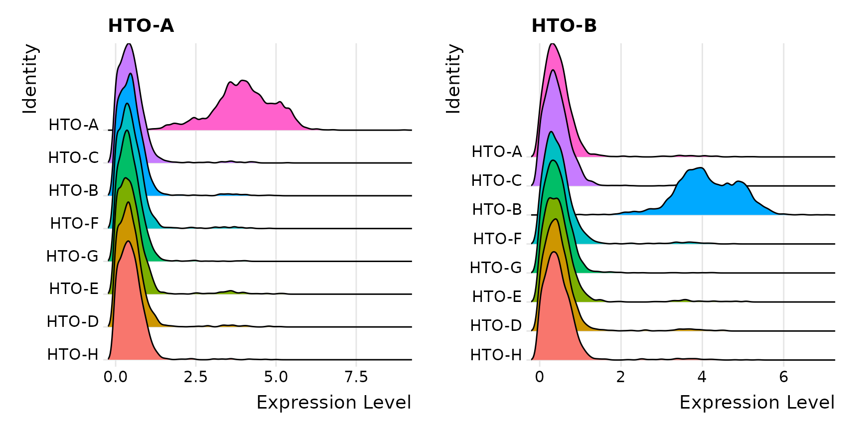

Visualize pairs of HTO signals to confirm mutual exclusivity in singlets

FeatureScatter(pbmc.hashtag, feature1 = "hto_HTO-A", feature2 = "hto_HTO-B")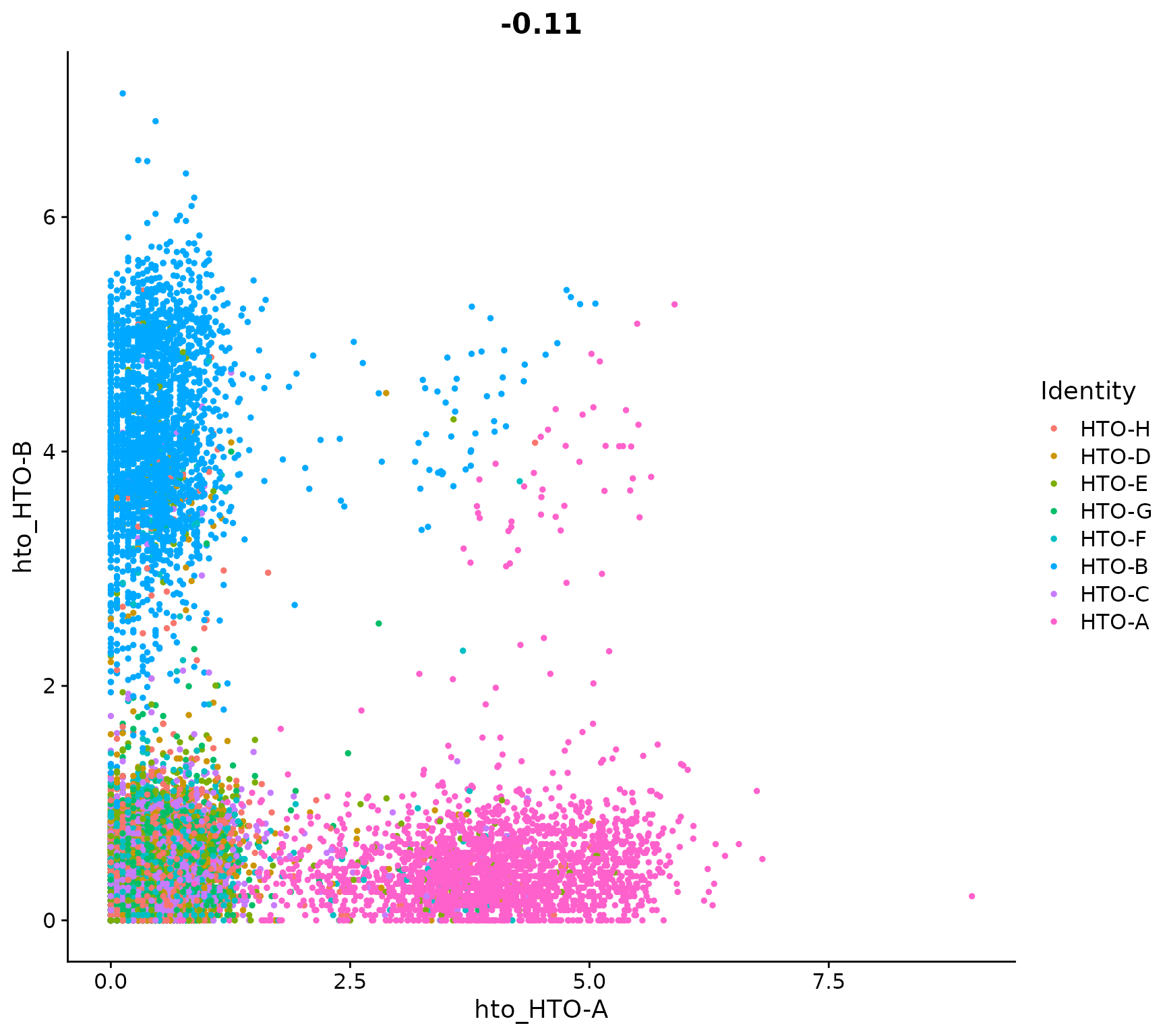

Compare number of UMIs for singlets, doublets and negative cells

Idents(pbmc.hashtag) <- "HTO_classification.global"
VlnPlot(pbmc.hashtag, features = "nCount_RNA", pt.size = 0.1, log = TRUE)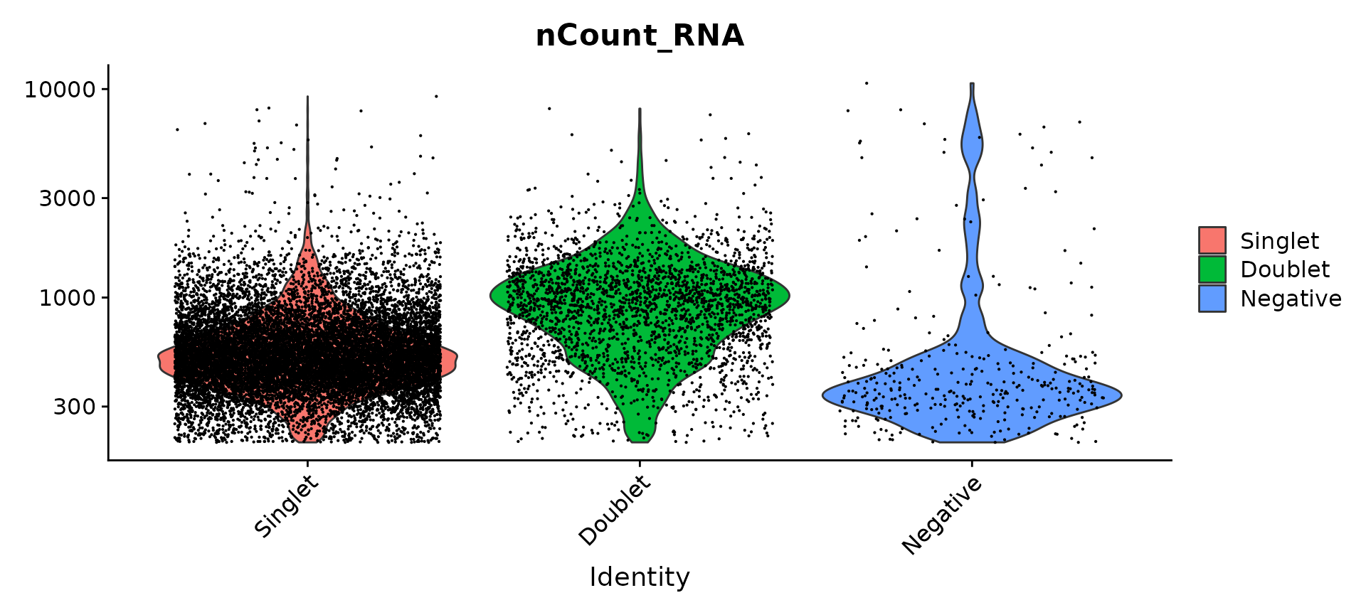

Generate a two dimensional tSNE embedding for HTOs. Here we are grouping cells by singlets and doublets for simplicity.

# First, we will remove negative cells from the object
pbmc.hashtag.subset <- subset(pbmc.hashtag, idents = "Negative", invert = TRUE)

# Calculate a tSNE embedding of the HTO data
DefaultAssay(pbmc.hashtag.subset) <- "HTO"
pbmc.hashtag.subset <- ScaleData(pbmc.hashtag.subset, features = rownames(pbmc.hashtag.subset),
    verbose = FALSE)
pbmc.hashtag.subset <- RunPCA(pbmc.hashtag.subset, features = rownames(pbmc.hashtag.subset), approx = FALSE)
pbmc.hashtag.subset <- RunTSNE(pbmc.hashtag.subset, dims = 1:8, perplexity = 100)
DimPlot(pbmc.hashtag.subset)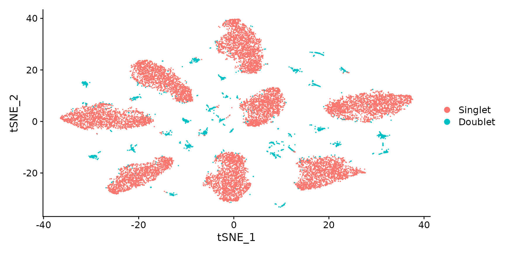

# You can also visualize the more detailed classification result by running Idents(object) <-
# 'HTO_classification' before plotting. Here, you can see that each of the small clouds on the
# tSNE plot corresponds to one of the 28 possible doublet combinations.

Create an HTO heatmap, based on Figure 1C in the Cell Hashing paper.

# To increase the efficiency of plotting, you can subsample cells using the num.cells argument
HTOHeatmap(pbmc.hashtag, assay = "HTO", ncells = 5000)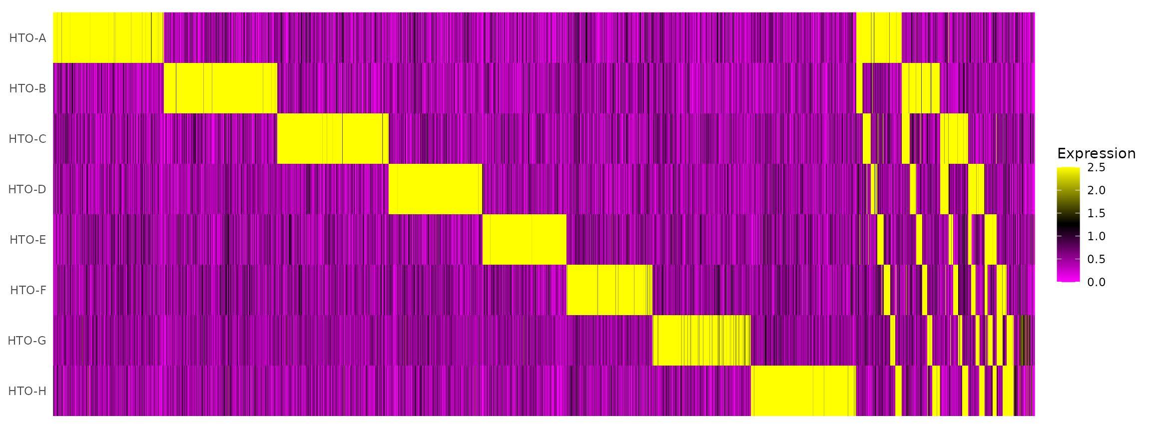

Cluster and visualize cells using the usual scRNA-seq workflow, and examine for the potential presence of batch effects.

# Extract the singlets
pbmc.singlet <- subset(pbmc.hashtag, idents = "Singlet")

# Select the top 1000 most variable features
pbmc.singlet <- FindVariableFeatures(pbmc.singlet, selection.method = "mean.var.plot")

# Scaling RNA data, we only scale the variable features here for efficiency
pbmc.singlet <- ScaleData(pbmc.singlet, features = VariableFeatures(pbmc.singlet))

# Run PCA
pbmc.singlet <- RunPCA(pbmc.singlet, features = VariableFeatures(pbmc.singlet))

# We select the top 10 PCs for clustering and tSNE based on PCElbowPlot
pbmc.singlet <- FindNeighbors(pbmc.singlet, reduction = "pca", dims = 1:10)
pbmc.singlet <- FindClusters(pbmc.singlet, resolution = 0.6, verbose = FALSE)
pbmc.singlet <- RunTSNE(pbmc.singlet, reduction = "pca", dims = 1:10)

# Projecting singlet identities on TSNE visualization
DimPlot(pbmc.singlet, group.by = "HTO_classification")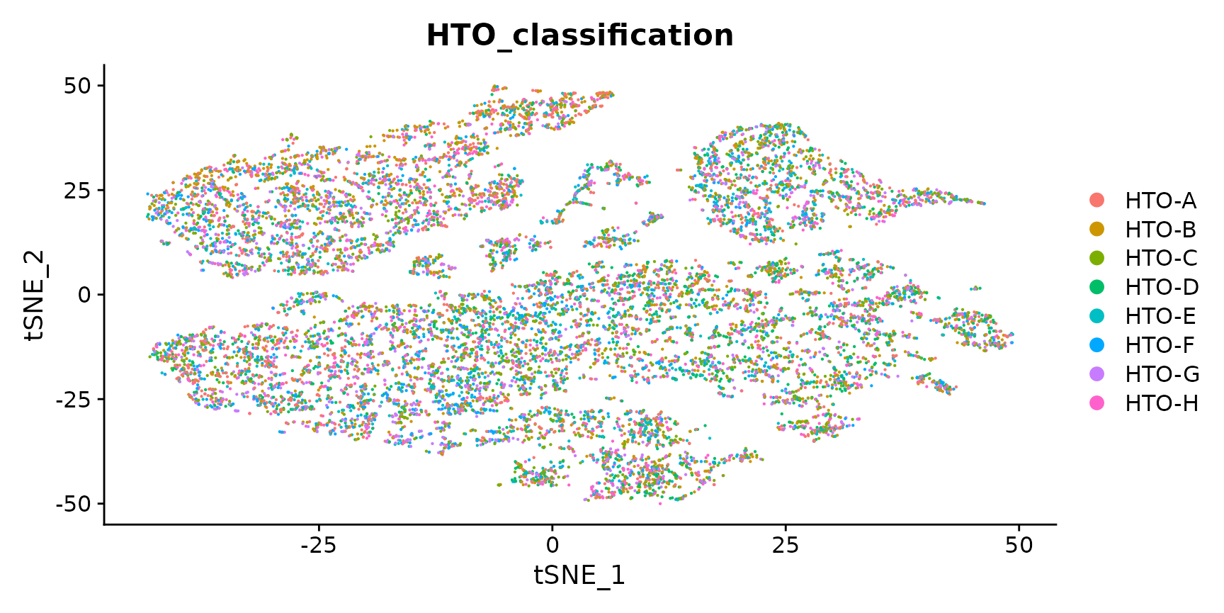

12-HTO dataset from four human cell lines

Dataset description:

Data represent single cells collected from four cell lines: HEK, K562, KG1 and THP1
Each cell line was further split into three samples (12 samples in total).
Each sample was labeled with a hashing antibody mixture (CD29 and CD45), pooled, and run on a single lane of 10X.
Based on this design, we should be able to detect doublets both across and within cell types
You can download the count matrices for RNA and HTO here, and are available on GEO here

Create Seurat object, add HTO data and perform normalization

# Read in UMI count matrix for RNA
hto12.umis <- readRDS("/brahms/shared/vignette-data/hto12_umi_mtx.rds")

# Read in HTO count matrix
hto12.htos <- readRDS("/brahms/shared/vignette-data/hto12_hto_mtx.rds")

# Select cell barcodes detected in both RNA and HTO
cells.use <- intersect(rownames(hto12.htos), colnames(hto12.umis))

# Create Seurat object and add HTO data
hto12 <- CreateSeuratObject(counts = Matrix::Matrix(as.matrix(hto12.umis[, cells.use]), sparse = T),
    min.features = 300)
hto12[["HTO"]] <- CreateAssayObject(counts = t(x = hto12.htos[colnames(hto12), 1:12]))

# Normalize data
hto12 <- NormalizeData(hto12)
hto12 <- NormalizeData(hto12, assay = "HTO", normalization.method = "CLR")

Demultiplex data

hto12 <- HTODemux(hto12, assay = "HTO", positive.quantile = 0.99)

Visualize demultiplexing results

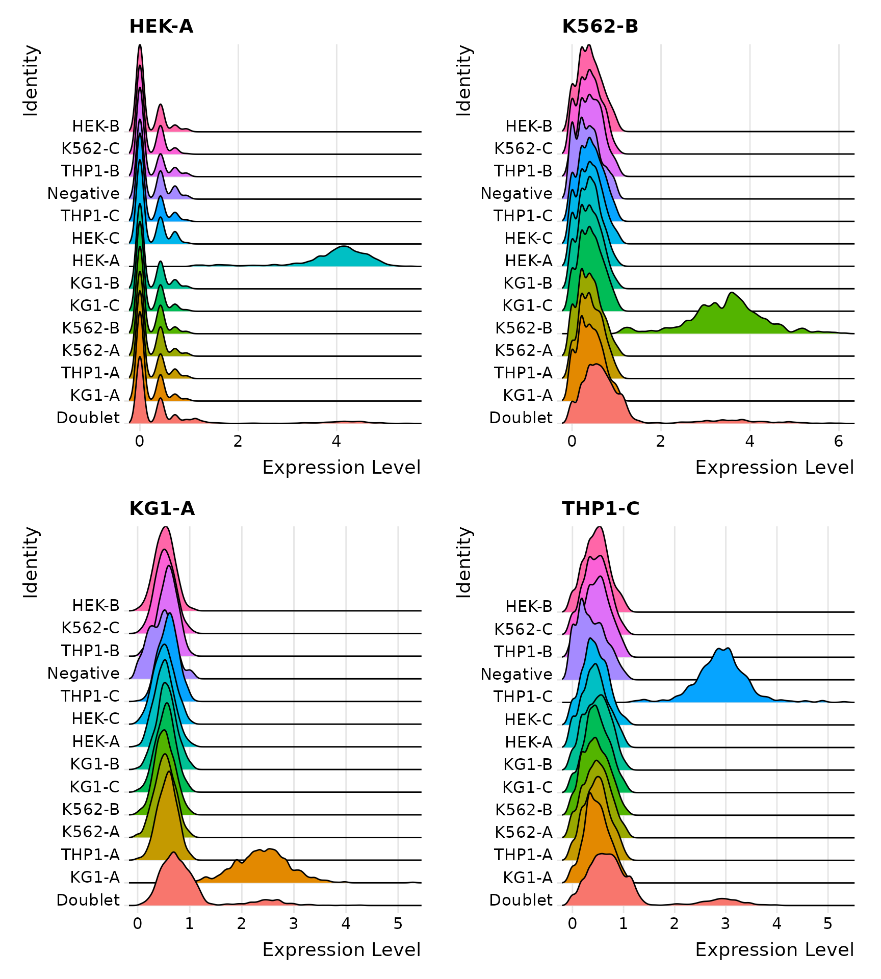
Distribution of selected HTOs grouped by classification, displayed by ridge plots

RidgePlot(hto12, assay = "HTO", features = c("HEK-A", "K562-B", "KG1-A", "THP1-C"), ncol = 2)

Visualize HTO signals in a heatmap

HTOHeatmap(hto12, assay = "HTO")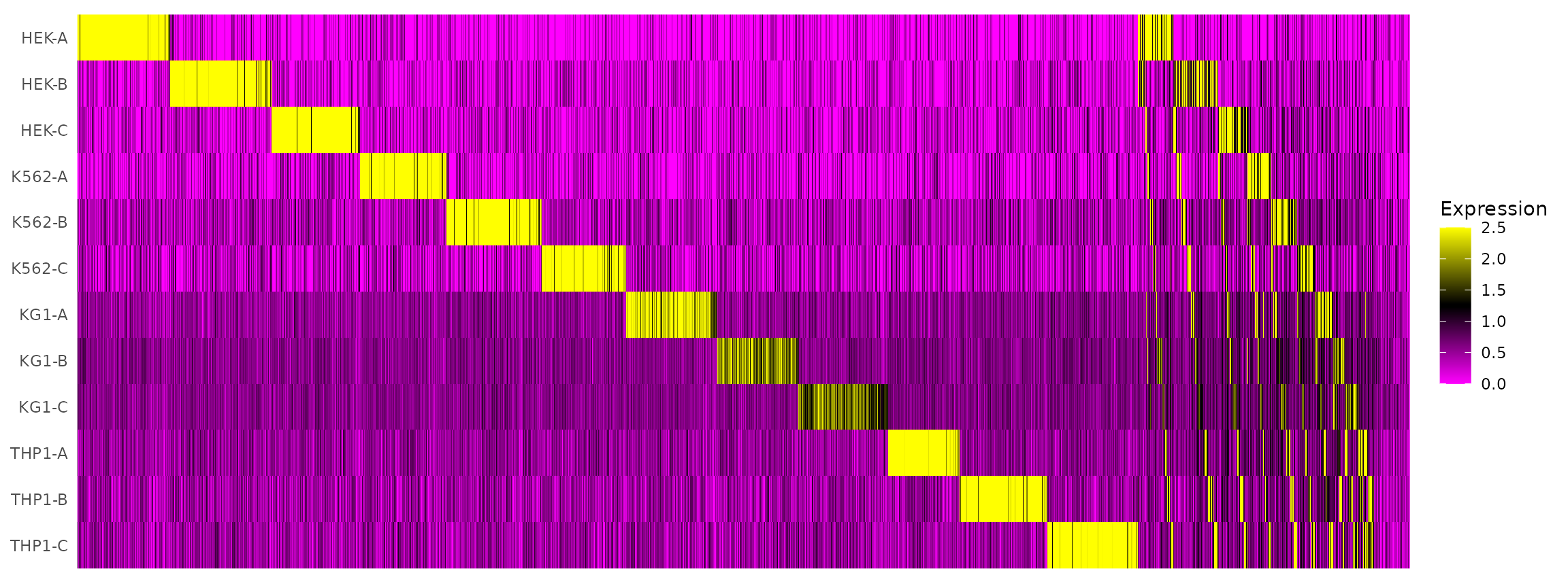

Visualize RNA clustering

Below, we cluster the cells using our standard scRNA-seq workflow. As expected we see four major clusters, corresponding to the cell lines

In addition, we see small clusters in between, representing mixed transcriptomes that are correctly annotated as doublets.

We also see within-cell type doublets, that are (perhaps unsurprisingly) intermixed with singlets of the same cell type

# Remove the negative cells
hto12 <- subset(hto12, idents = "Negative", invert = TRUE)

# Run PCA on most variable features
hto12 <- FindVariableFeatures(hto12, selection.method = "mean.var.plot")
hto12 <- ScaleData(hto12, features = VariableFeatures(hto12))
hto12 <- RunPCA(hto12)
hto12 <- RunTSNE(hto12, dims = 1:5, perplexity = 100)
DimPlot(hto12) + NoLegend()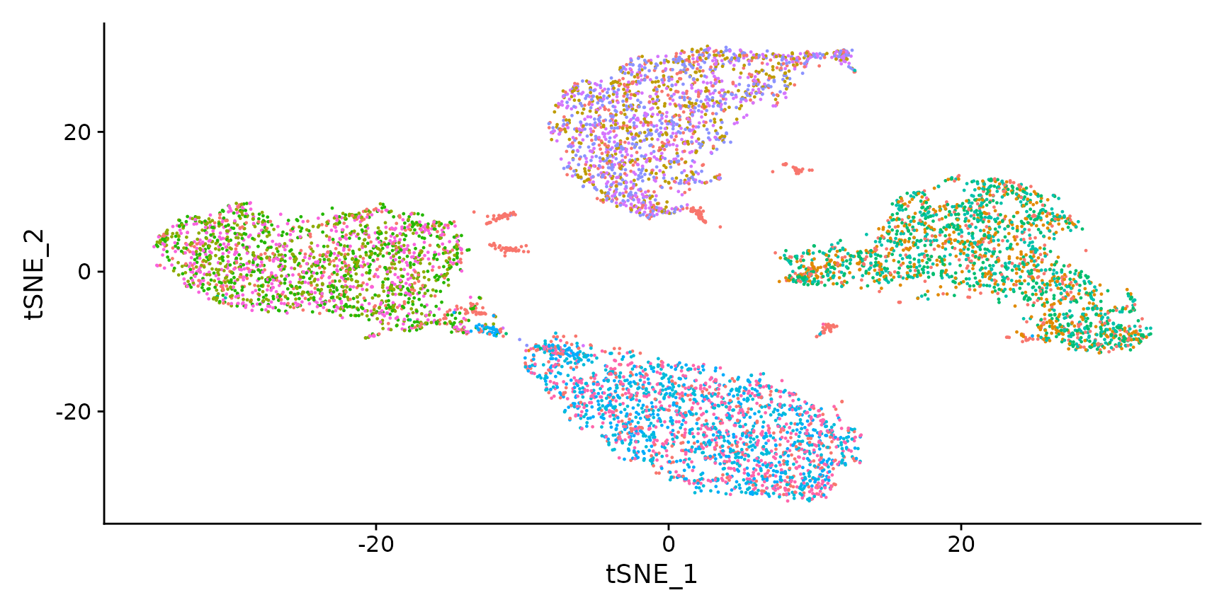

Session Info

sessionInfo()

## R version 4.5.2 (2025-10-31)
## Platform: x86_64-pc-linux-gnu
## Running under: Ubuntu 24.04.4 LTS
## 
## Matrix products: default
## BLAS:   /usr/lib/x86_64-linux-gnu/openblas-pthread/libblas.so.3 
## LAPACK: /usr/lib/x86_64-linux-gnu/openblas-pthread/libopenblasp-r0.3.26.so;  LAPACK version 3.12.0
## 
## locale:
##  [1] LC_CTYPE=en_US.UTF-8       LC_NUMERIC=C              
##  [3] LC_TIME=en_US.UTF-8        LC_COLLATE=en_US.UTF-8    
##  [5] LC_MONETARY=en_US.UTF-8    LC_MESSAGES=en_US.UTF-8   
##  [7] LC_PAPER=en_US.UTF-8       LC_NAME=C                 
##  [9] LC_ADDRESS=C               LC_TELEPHONE=C            
## [11] LC_MEASUREMENT=en_US.UTF-8 LC_IDENTIFICATION=C       
## 
## time zone: Etc/UTC
## tzcode source: system (glibc)
## 
## attached base packages:
## [1] stats     graphics  grDevices utils     datasets  methods   base     
## 
## other attached packages:
## [1] future_1.70.0      Seurat_5.5.0       SeuratObject_5.4.0 sp_2.2-1          
## 
## loaded via a namespace (and not attached):
##   [1] RColorBrewer_1.1-3     jsonlite_2.0.0         magrittr_2.0.5        
##   [4] spatstat.utils_3.2-2   ggbeeswarm_0.7.3       farver_2.1.2          
##   [7] rmarkdown_2.30         fs_2.1.0               ragg_1.5.1            
##  [10] vctrs_0.7.1            ROCR_1.0-12            spatstat.explore_3.8-0
##  [13] htmltools_0.5.9        sass_0.4.10            sctransform_0.4.3     
##  [16] parallelly_1.47.0      KernSmooth_2.23-26     bslib_0.10.0          
##  [19] htmlwidgets_1.6.4      desc_1.4.3             ica_1.0-3             
##  [22] plyr_1.8.9             plotly_4.12.0          zoo_1.8-15            
##  [25] cachem_1.1.0           igraph_2.3.0           mime_0.13             
##  [28] lifecycle_1.0.5        pkgconfig_2.0.3        Matrix_1.7-5          
##  [31] R6_2.6.1               fastmap_1.2.0          fitdistrplus_1.2-6    
##  [34] shiny_1.13.0           digest_0.6.39          patchwork_1.3.2       
##  [37] tensor_1.5.1           RSpectra_0.16-2        irlba_2.3.7           
##  [40] textshaping_1.0.5      labeling_0.4.3         progressr_0.19.0      
##  [43] spatstat.sparse_3.1-0  httr_1.4.8             polyclip_1.10-7       
##  [46] abind_1.4-8            compiler_4.5.2         withr_3.0.2           
##  [49] S7_0.2.1               fastDummies_1.7.6      MASS_7.3-65           
##  [52] tools_4.5.2            vipor_0.4.7            lmtest_0.9-40         
##  [55] otel_0.2.0             beeswarm_0.4.0         httpuv_1.6.16         
##  [58] future.apply_1.20.2    goftest_1.2-3          glue_1.8.0            
##  [61] nlme_3.1-168           promises_1.5.0         grid_4.5.2            
##  [64] Rtsne_0.17             cluster_2.1.8.2        reshape2_1.4.5        
##  [67] generics_0.1.4         gtable_0.3.6           spatstat.data_3.1-9   
##  [70] tidyr_1.3.2            data.table_1.18.2.1    spatstat.geom_3.7-3   
##  [73] RcppAnnoy_0.0.23       ggrepel_0.9.8          RANN_2.6.2            
##  [76] pillar_1.11.1          stringr_1.6.0          spam_2.11-3           
##  [79] RcppHNSW_0.6.0         later_1.4.8            splines_4.5.2         
##  [82] dplyr_1.2.0            lattice_0.22-7         survival_3.8-3        
##  [85] deldir_2.0-4           tidyselect_1.2.1       miniUI_0.1.2          
##  [88] pbapply_1.7-4          knitr_1.51             gridExtra_2.3         
##  [91] scattermore_1.2        xfun_0.56              matrixStats_1.5.0     
##  [94] stringi_1.8.7          lazyeval_0.2.3         yaml_2.3.12           
##  [97] evaluate_1.0.5         codetools_0.2-20       tibble_3.3.1          
## [100] cli_3.6.6              uwot_0.2.4             xtable_1.8-8          
## [103] reticulate_1.46.0      systemfonts_1.3.2      jquerylib_0.1.4       
## [106] Rcpp_1.1.1-1.1         globals_0.19.1         spatstat.random_3.4-5 
## [109] png_0.1-9              ggrastr_1.0.2          spatstat.univar_3.1-7 
## [112] parallel_4.5.2         pkgdown_2.2.0          ggplot2_4.0.3         
## [115] dotCall64_1.2          listenv_0.10.1         viridisLite_0.4.3     
## [118] scales_1.4.0           ggridges_0.5.7         purrr_1.2.1           
## [121] rlang_1.2.0            cowplot_1.2.0          formatR_1.14

Compiled: 2026-05-22

8-HTO dataset from human PBMCs

Basic setup

Adding HTO data as an independent assay

Demultiplex cells based on HTO enrichment

Visualize demultiplexing results

12-HTO dataset from four human cell lines

Create Seurat object, add HTO data and perform normalization

Demultiplex data

Visualize demultiplexing results

Visualize RNA clustering