Analysis of Image-based Spatial Data in Seurat
Compiled: April 28, 2026
Source:vignettes/seurat5_spatial_vignette_2.Rmd
seurat5_spatial_vignette_2.RmdOverview
In this vignette, we introduce a Seurat extension to analyze new types of spatially-resolved data. We have previously introduced a spatial framework which is compatible with sequencing-based technologies, like the 10x Genomics Visium system, or SLIDE-seq. Here, we extend this framework to analyze new data types that are captured via highly multiplexed imaging. In contrast to sequencing-based technologies, these datasets are often targeted (i.e. they profile a pre-selected set of genes). However they can resolve individual molecules - retaining single-cell (and subcellular) resolution. These approaches also often capture cellular boundaries (segmentations).
We update the Seurat infrastructure to enable the analysis, visualization, and exploration of these exciting datasets. In this vignette, we focus on three datasets produced by different multiplexed imaging technologies, each of which is publicly available. We will be adding support for additional imaging-based technologies in the coming months.
- Vizgen MERSCOPE (Mouse Brain)
- Nanostring CosMx Spatial Molecular Imager (FFPE Human Lung)
- Akoya CODEX (Human Lymph Node)
First, we load the packages necessary for this vignette.
Mouse Brain: Vizgen MERSCOPE
This dataset was produced using the Vizgen MERSCOPE system, which utilizes the MERFISH technology. The total dataset is available for public download, and contains nine samples (three full coronal slices of the mouse brain, with three biological replicates per slice). The gene panel consists of 483 gene targets, representing known anonical cell type markers, nonsensory G-Protein coupled receptors (GPCRs), and Receptor Tyrosine Kinases (RTKs). In this vignette, we analyze one of the samples - slice 2, replicate 1. The median number of transcripts detected in each cell is 206.
First, we read in the dataset and create a Seurat object.
We use the LoadVizgen() function, which we have written
to read in the output of the Vizgen analysis pipeline. The resulting
Seurat object contains the following information:
- A count matrix, indicating the number of observed molecules for each of the 483 transcripts in each cell. This matrix is analogous to a count matrix in scRNA-seq, and is stored by default in the RNA assay of the Seurat object
# Loading segmentations is a slow process and multi processing with the future pacakge is
# recommended
vizgen.obj <- LoadVizgen(data.dir = "/brahms/hartmana/vignette_data/vizgen/s2r1/", fov = "s2r1")
The next pieces of information are specific to imaging assays, and is stored in the images slot of the resulting Seurat object:
Cell Centroids: The spatial coordinates marking the centroid for each cell being profiled
# Get the center position of each centroid. There is one row per cell in this dataframe.
head(GetTissueCoordinates(vizgen.obj[["s2r1"]][["centroids"]]))
## x y cell
## 1 638.5640 4594.216 149164679103246548309819743981609972453
## 2 593.8034 4516.240 215843146921706462965382248182021894607
## 3 597.3134 4566.676 230248905804673613678286091156141465134
## 4 613.2434 4609.498 237155298815097057940587033798543926454
## 5 609.1934 4603.180 256099454901769634241742157204636917386
## 6 623.8814 4642.708 52442222147121971758529793775250916001Cell Segmentation Boundaries: The spatial coordinates that describe the polygon segmentation of each single cell
# Get the coordinates for each segmentation vertice. Each cell will have a variable number of
# vertices describing its shape.
head(GetTissueCoordinates(vizgen.obj[["s2r1"]][["segmentation"]]))
## x y cell
## 1 644.0774 4589.022 149164679103246548309819743981609972453
## 2 643.9694 4589.022 149164679103246548309819743981609972453
## 3 643.8614 4589.022 149164679103246548309819743981609972453
## 4 643.7642 4588.924 149164679103246548309819743981609972453
## 5 643.7534 4588.914 149164679103246548309819743981609972453
## 6 643.6454 4588.914 149164679103246548309819743981609972453Molecule positions: The spatial coordinates for each individual molecule that was detected during the multiplexed smFISH experiment.
# Fetch molecules positions for Chrm1
head(FetchData(vizgen.obj[["s2r1"]][["molecules"]], vars = "Chrm1"))
## x y molecule
## 1 577.3373 4205.977 Chrm1
## 2 600.0218 3917.781 Chrm1
## 3 508.2736 3934.063 Chrm1
## 4 630.7590 3948.586 Chrm1
## 5 635.1143 3969.567 Chrm1
## 6 582.7043 4021.577 Chrm1Preprocessing and unsupervised analysis
We start by performing a standard unsupervised clustering analysis, essentially first treating the dataset as an scRNA-seq experiment. We use SCTransform-based normalization, though we slightly modify the default clipping parameters to mitigate the effect of outliers that we occasionally observe in smFISH experiments. After normalization, we can run dimensional reduction and clustering.
vizgen.obj <- SCTransform(vizgen.obj, assay = "Vizgen", clip.range = c(-10, 10))
vizgen.obj <- RunPCA(vizgen.obj, npcs = 30, features = rownames(vizgen.obj))
vizgen.obj <- RunUMAP(vizgen.obj, dims = 1:30)
vizgen.obj <- FindNeighbors(vizgen.obj, reduction = "pca", dims = 1:30)
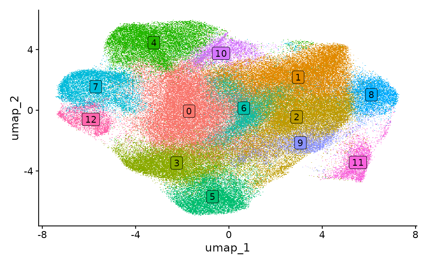
vizgen.obj <- FindClusters(vizgen.obj, resolution = 0.3)We can then visualize the results of the clustering either in UMAP
space (with DimPlot()) or overlaid on the image with
ImageDimPlot().
DimPlot(vizgen.obj, reduction = "umap")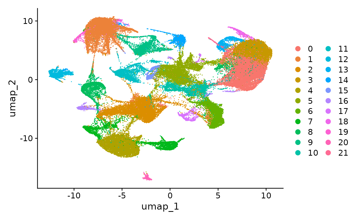
ImageDimPlot(vizgen.obj, fov = "s2r1", cols = "polychrome", axes = TRUE)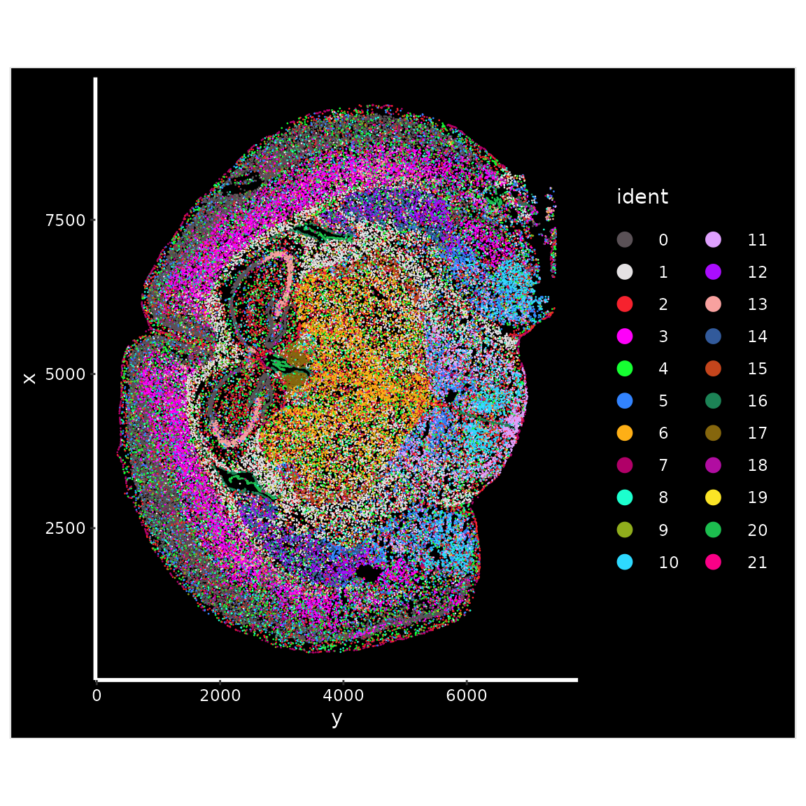
You can also customize multiple aspect of the plot, including the color scheme, cell border widths, and size (see below).
Customizing spatial plots in Seurat
The ImageDimPlot() and ImageFeaturePlot()
functions have a few parameters which you can customize individual
visualizations. These include:
- alpha: Ranges from 0 to 1. Sets the transparency of within-cell coloring.
- size: determines the size of points representing cells, if centroids are being plotted
- cols: Sets the color scheme for the internal shading of each cell.
Examples settings are
polychrome,glasbey,Paired,Set3, andparade. Default is the ggplot2 color palette - shuffle.cols: In some cases the selection of
colsis more effective when the same colors are assigned to different clusters. Setshuffle.cols = TRUEto randomly shuffle the colors in the palette. - border.size: Sets the width of the cell segmentation borders. By default, segmentations are plotted with a border size of 0.3 and centroids are plotted without border.
- border.color: Sets the color of the cell segmentation borders
- dark.background: Sets a black background color (TRUE by default)
- axes: Display
Since it can be difficult to visualize the spatial localization patterns of an individual cluster when viewing them all together, we can highlight all cells that belong to a particular cluster:
p1 <- ImageDimPlot(vizgen.obj, fov = "s2r1", cols = "red", cells = WhichCells(vizgen.obj, idents = 1))
p2 <- ImageDimPlot(vizgen.obj, fov = "s2r1", cols = "red", cells = WhichCells(vizgen.obj, idents = 15))
p1 + p2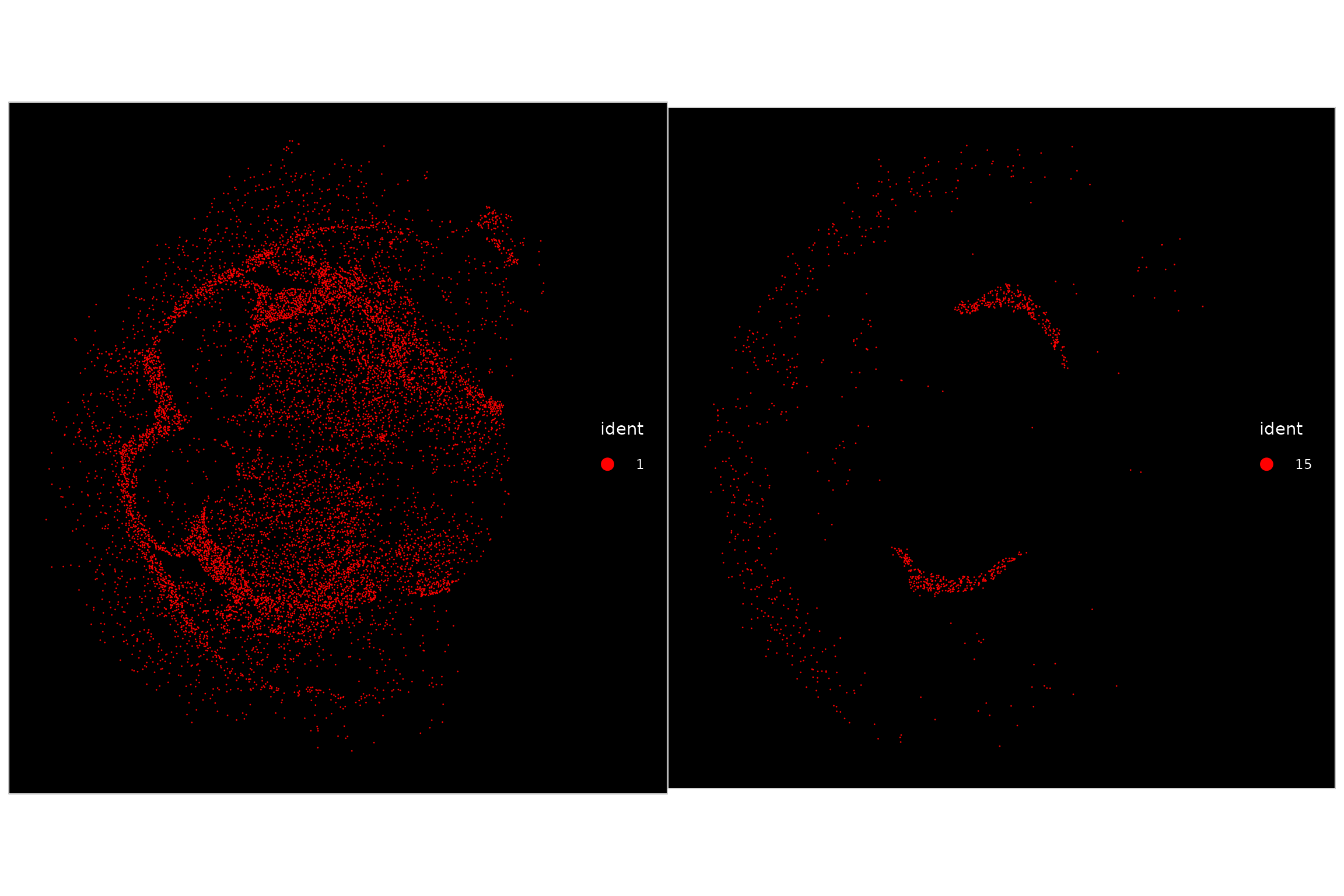
We can find markers of individual clusters and visualize their
spatial expression pattern. We can color cells based on their quantified
expression of an individual gene, using ImageFeaturePlot(),
which is analagous to the FeaturePlot() function for
visualizing expression on a 2D embedding. Since MERFISH images
individual molecules, we can also visualize the location of individual
molecules.
p1 <- ImageFeaturePlot(vizgen.obj, features = "Slc17a7")
p2 <- ImageDimPlot(vizgen.obj, molecules = "Slc17a7", nmols = 10000, alpha = 0.3, mols.cols = "red")
p1 + p2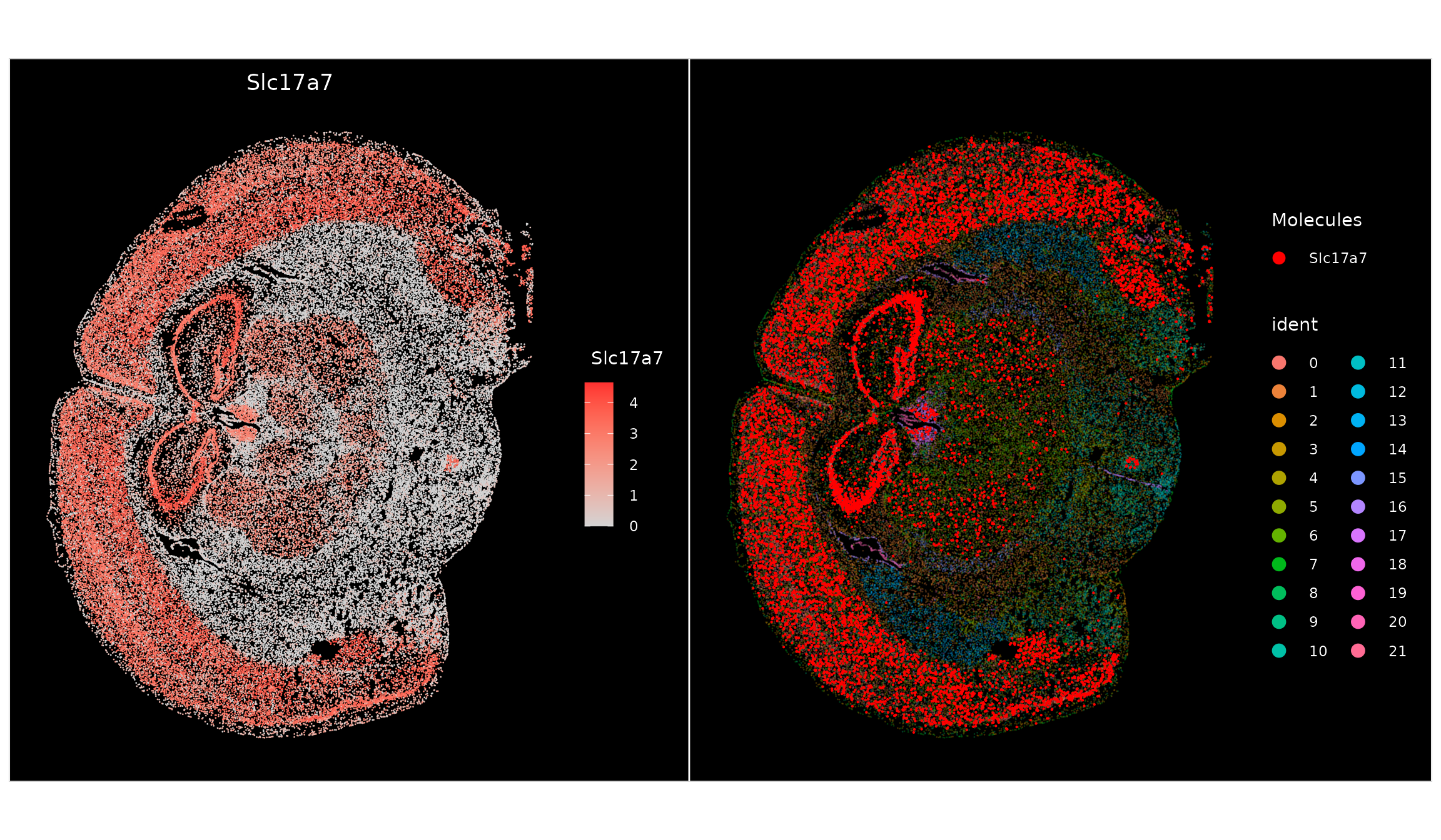
Note that the nmols parameter can be used to reduce the
total number of molecules shown to reduce overplotting. You can also use
the mols.size, mols.cols, and
mols.alpha parameter to further optimize.
Plotting molecules is especially useful for visualizing co-expression of multiple genes on the same plot.
p1 <- ImageDimPlot(vizgen.obj, fov = "s2r1", alpha = 0.3, molecules = c("Slc17a7", "Olig1"), nmols = 10000)
markers.14 <- FindMarkers(vizgen.obj, ident.1 = "14")
p2 <- ImageDimPlot(vizgen.obj, fov = "s2r1", alpha = 0.3, molecules = rownames(markers.14)[1:4],
    nmols = 10000)
p1 + p2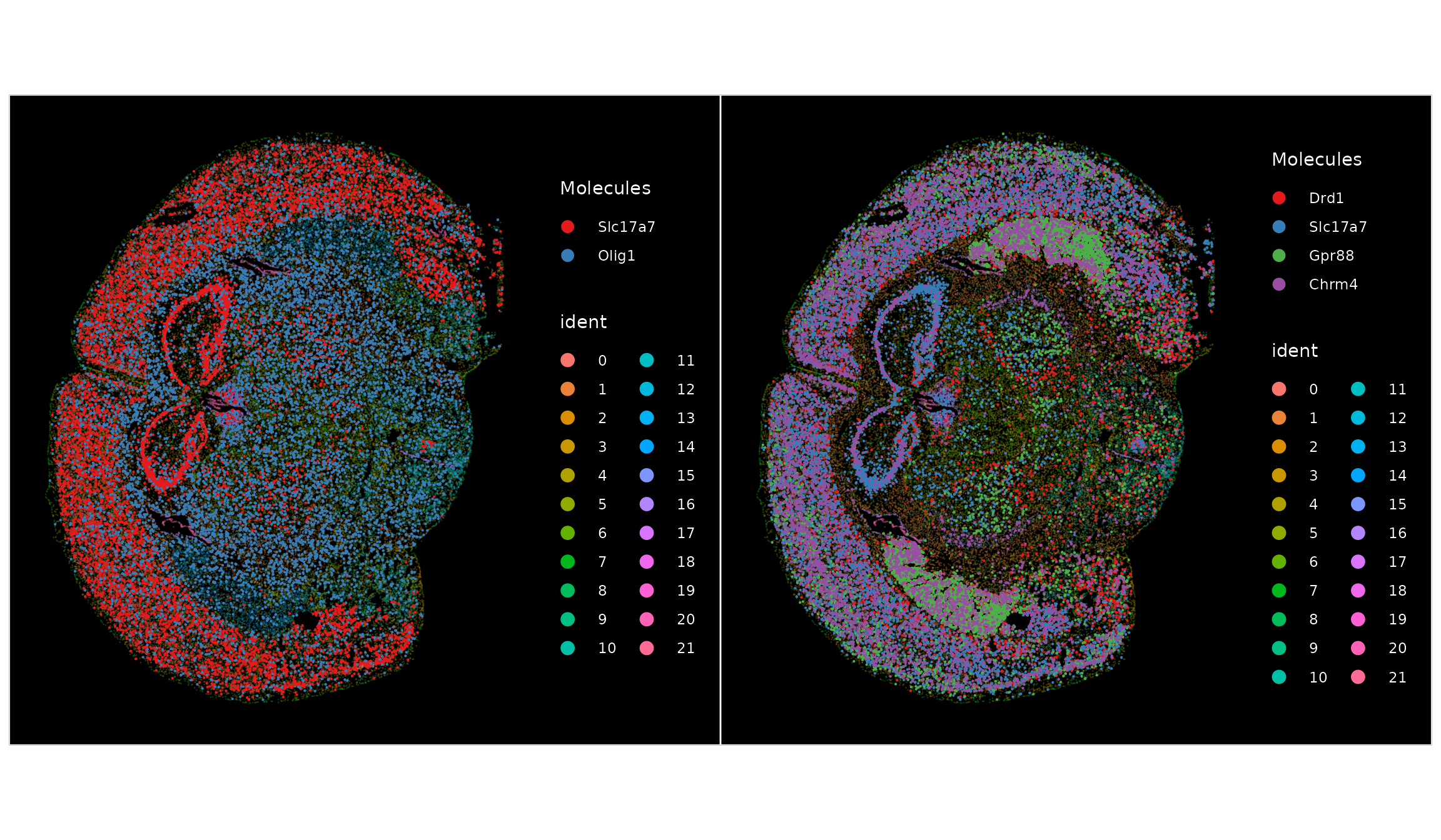
The updated Seurat spatial framework has the option to treat cells as individual points, or also to visualize cell boundaries (segmentations). By default, Seurat ignores cell segmentations and treats each cell as a point (‘centroids’). This speeds up plotting, especially when looking at large areas, where cell boundaries are too small to visualize.
We can zoom into a region of tissue, creating a new field of view.
For example, we can zoom into a region that contains the hippocampus.
Once zoomed-in, we can set DefaultBoundary() to show cell
segmentations. You can also ‘simplify’ the cell segmentations, reducing
the number of edges in each polygon to speed up plotting.
# create a Crop
cropped.coords <- Crop(vizgen.obj[["s2r1"]], x = c(1750, 3000), y = c(3750, 5250), coords = "plot")
# set a new field of view (fov)
vizgen.obj[["hippo"]] <- cropped.coords

# visualize FOV using default settings (no cell boundaries)
p1 <- ImageDimPlot(vizgen.obj, fov = "hippo", axes = TRUE, size = 0.7, border.color = "white", cols = "polychrome",
    coord.fixed = FALSE)

# visualize FOV with full cell segmentations
DefaultBoundary(vizgen.obj[["hippo"]]) <- "segmentation"
p2 <- ImageDimPlot(vizgen.obj, fov = "hippo", axes = TRUE, border.color = "white", border.size = 0.1,
    cols = "polychrome", coord.fixed = FALSE)

# simplify cell segmentations
vizgen.obj[["hippo"]][["simplified.segmentations"]] <- Simplify(coords = vizgen.obj[["hippo"]][["segmentation"]],
    tol = 3)
DefaultBoundary(vizgen.obj[["hippo"]]) <- "simplified.segmentations"

# visualize FOV with simplified cell segmentations
DefaultBoundary(vizgen.obj[["hippo"]]) <- "simplified.segmentations"
p3 <- ImageDimPlot(vizgen.obj, fov = "hippo", axes = TRUE, border.color = "white", border.size = 0.1,
    cols = "polychrome", coord.fixed = FALSE)

p1 + p2 + p3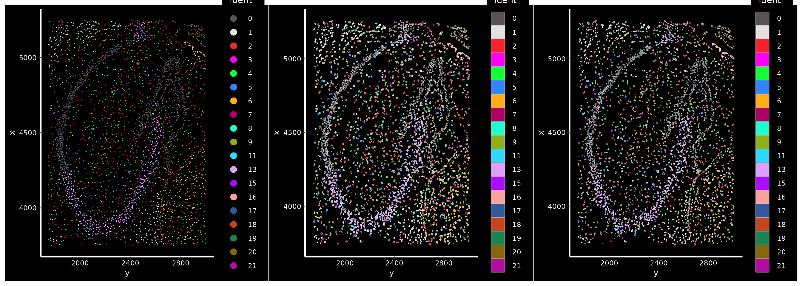
What is the tol parameter?
The tol parameter determines how simplified the resulting segmentations are. A higher value of tol will reduce the number of vertices more drastically which will speed up plotting, but some segmentation detail will be lost. See https://rgeos.r-forge.r-project.org/reference/topo-unary-gSimplify.html for examples using different values for tol.
We can visualize individual molecules plotted at higher resolution after zooming-in
# Since there is nothing behind the segmentations, alpha will slightly mute colors
ImageDimPlot(vizgen.obj, fov = "hippo", molecules = rownames(markers.14)[1:4], cols = "polychrome",
    mols.size = 1, alpha = 0.5, mols.cols = c("red", "blue", "yellow", "green"))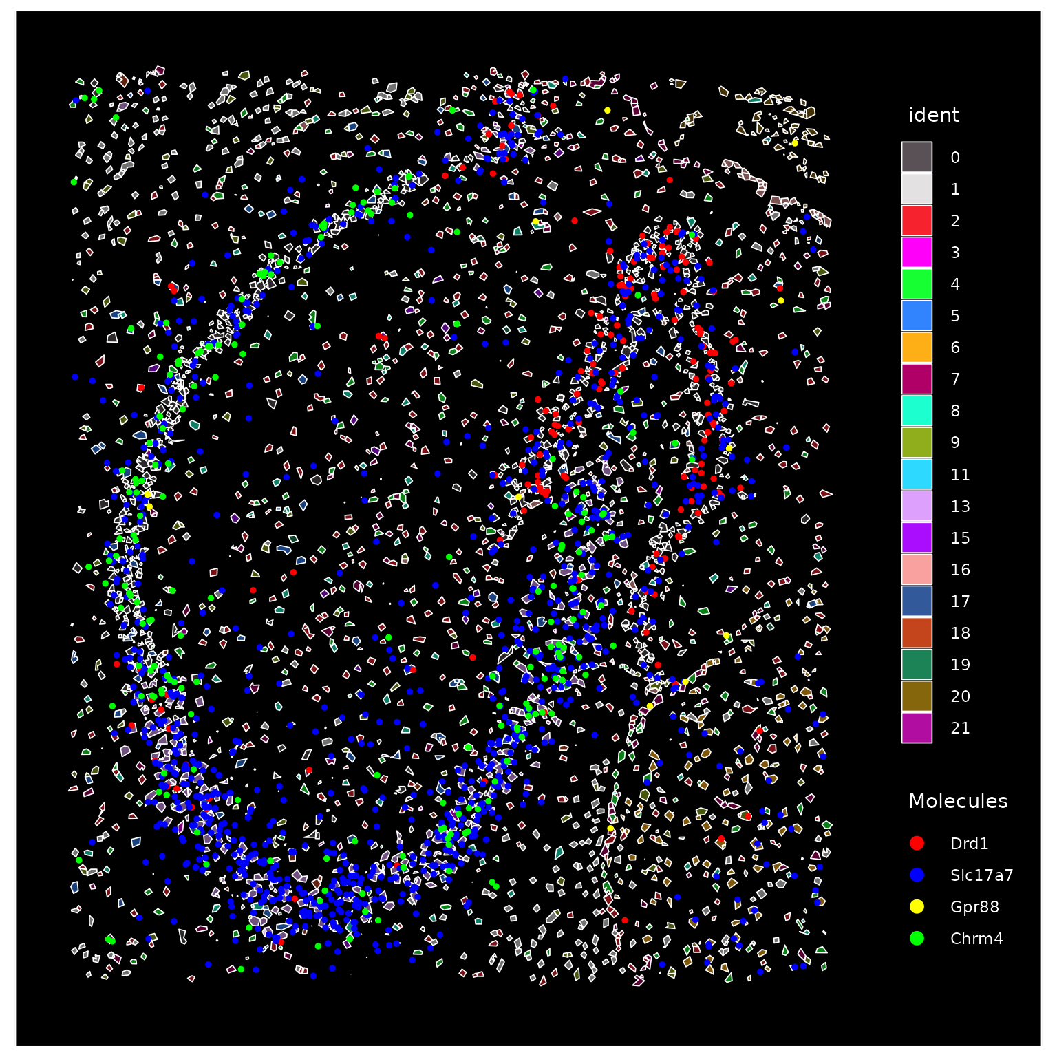
Mouse Brain: 10x Genomics Xenium In Situ
In this section we’ll analyze data produced by the Xenium platform. The vignette demonstrates how to load the per-transcript location data, cell x gene matrix, cell segmentation, and cell centroid information available in the Xenium outputs. The resulting Seurat object will contain the gene expression profile of each cell, the centroid and boundary of each cell, and the location of each individual detected transcript. The per-cell gene expression profiles are similar to standard single-cell RNA-seq and can be analyzed using the same tools.
This uses the Tiny subset dataset from 10x Genomics
provided in the Fresh
Frozen Mouse Brain for Xenium Explorer Demo which can be downloaded
as described below. These analysis steps are also compatible with the
larger Full coronal section, but will take longer to
execute.
wget https://cf.10xgenomics.com/samples/xenium/1.0.2/Xenium_V1_FF_Mouse_Brain_Coronal_Subset_CTX_HP/Xenium_V1_FF_Mouse_Brain_Coronal_Subset_CTX_HP_outs.zip
unzip Xenium_V1_FF_Mouse_Brain_Coronal_Subset_CTX_HP_outs.zip
First we read in the dataset and create a Seurat object. Provide the
path to the data folder for a Xenium run as the input path. The RNA data
is stored in the Xenium assay of the Seurat object. This
step should take about a minute (you can improve this by installing
arrow and hdf5r).
path <- "/brahms/hartmana/vignette_data/xenium_tiny_subset"
# Load the Xenium data
xenium.obj <- LoadXenium(path, fov = "fov", segmentations = "cell")
# remove cells with 0 counts
xenium.obj <- subset(xenium.obj, subset = nCount_Xenium > 0)
Spatial information is loaded into slots of the Seurat object,
labelled by the name of “field of view” (FOV) being loaded. Initially
all the data is loaded into the FOV named fov. Later, we
will make a cropped FOV that zooms into a region of interest.
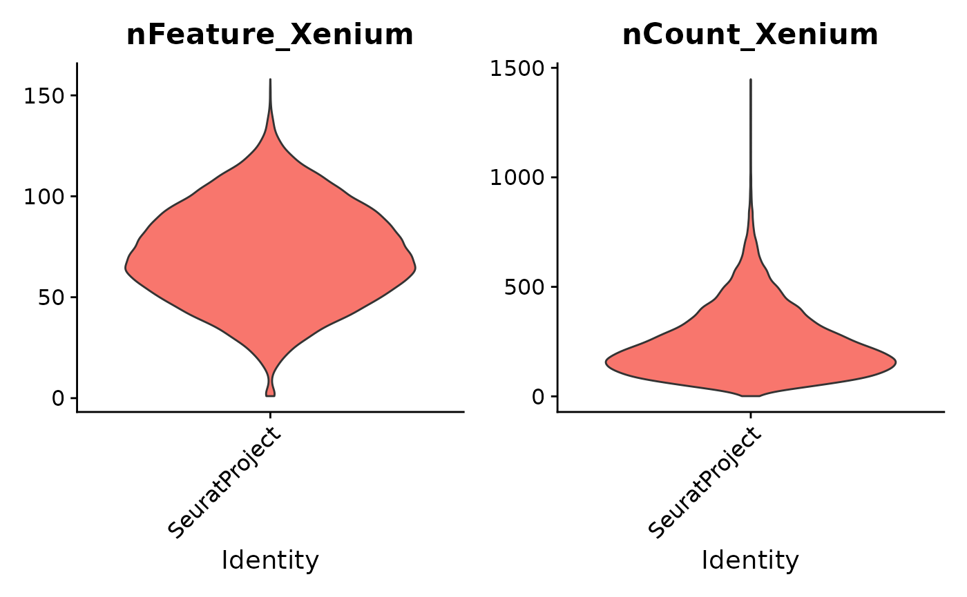
Standard QC plots provided by Seurat are available via the
Xenium assay. Here are violin plots of genes per cell
(nFeature_Xenium) and transcript counts per cell
(nCount_Xenium)
Next, we plot the positions of the pan-inhibitory neuron marker Gad1,
inhibitory neuron sub-type markers Pvalb, and Sst, and astrocyte marker
Gfap on the tissue using ImageDimPlot().
ImageDimPlot(xenium.obj, fov = "fov", molecules = c("Gad1", "Sst", "Pvalb", "Gfap"), nmols = 20000)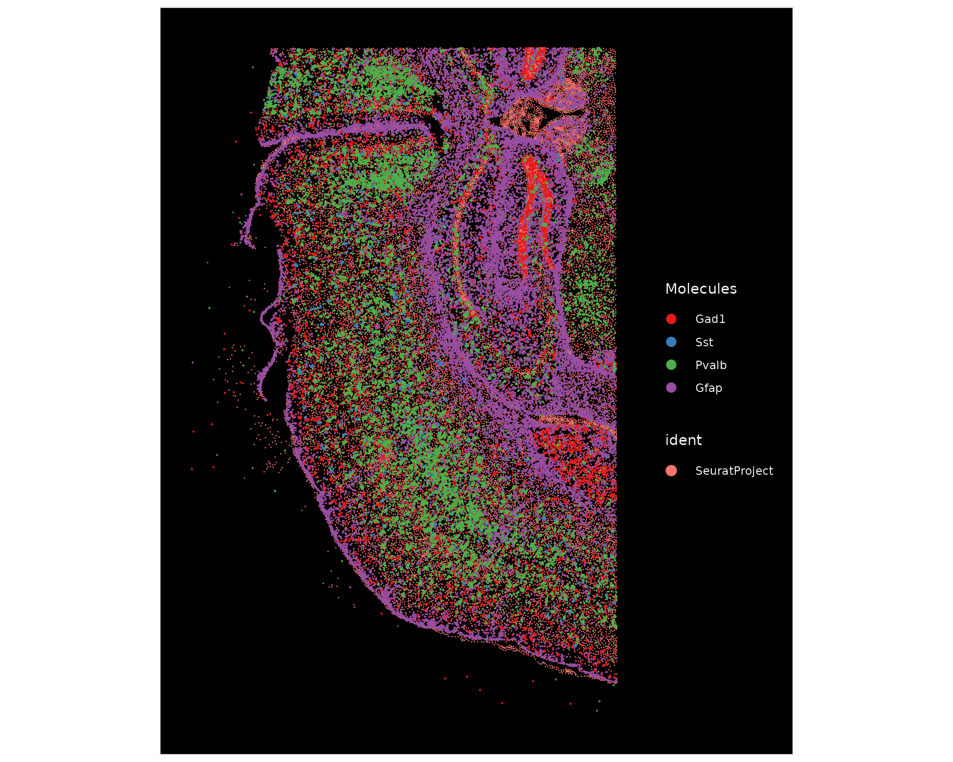
Here we visualize the expression level of some key layer marker genes
at the per-cell level using ImageFeaturePlot() which is
analogous to the FeaturePlot() function for visualizing
expression on a 2D embedding. We manually adjust the
max.cutoff for each gene to roughly the 90th percentile
(which can be specified with max.cutoff='q90') of it’s
count distribution to improve contrast.
ImageFeaturePlot(xenium.obj, features = c("Cux2", "Rorb", "Bcl11b", "Foxp2"), max.cutoff = c(25,
    35, 12, 10), size = 0.75, cols = c("white", "red"))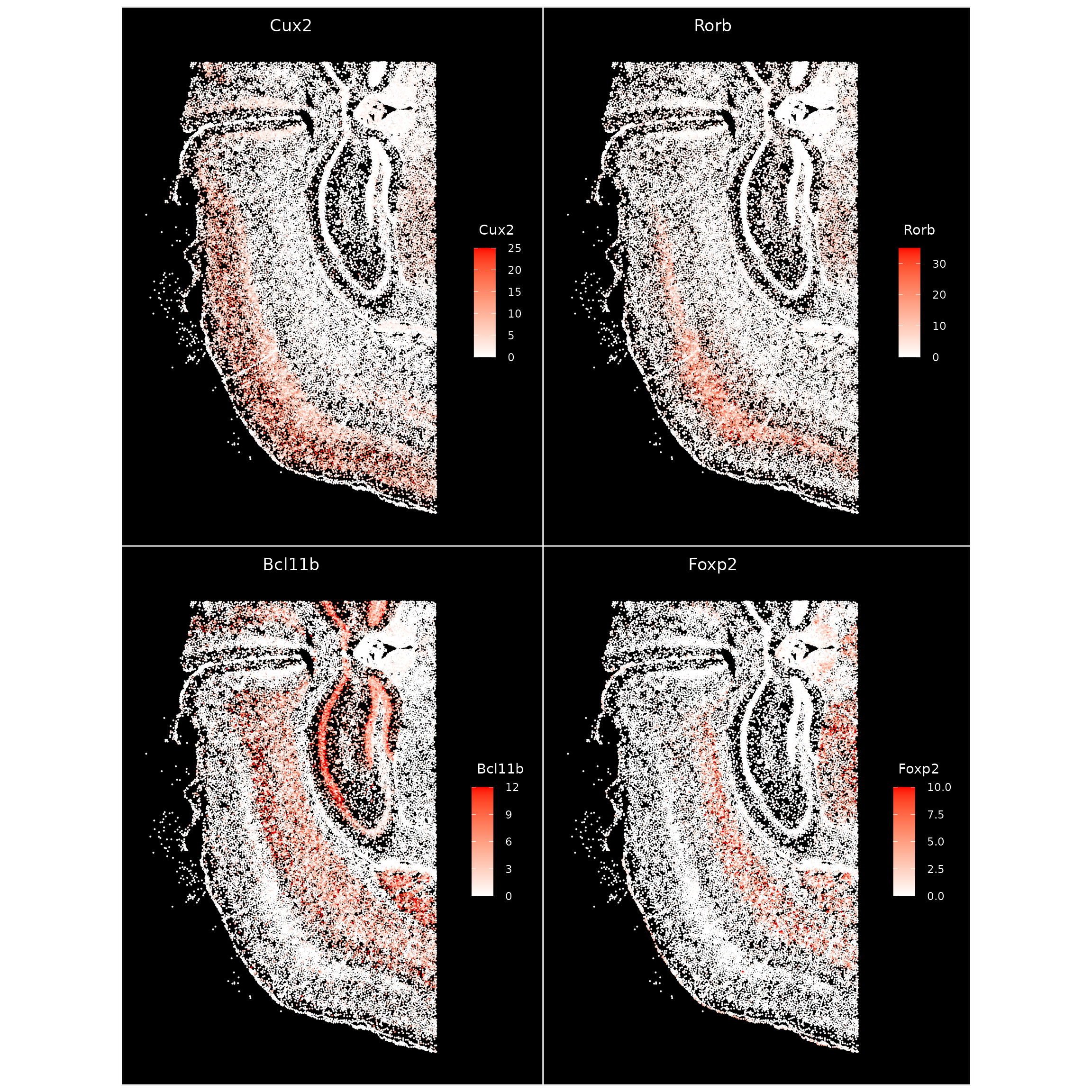
We can zoom in on a chosen area with the Crop()
function. Once zoomed-in, we can visualize cell segmentation boundaries
along with individual molecules.
cropped.coords <- Crop(xenium.obj[["fov"]], x = c(1200, 2900), y = c(3750, 4550), coords = "plot")
xenium.obj[["zoom"]] <- cropped.coords
# visualize cropped area with cell segmentations & selected molecules
DefaultBoundary(xenium.obj[["zoom"]]) <- "segmentation"
ImageDimPlot(xenium.obj, fov = "zoom", axes = TRUE, border.color = "white", border.size = 0.1, cols = "polychrome",
    coord.fixed = FALSE, molecules = c("Gad1", "Sst", "Npy2r", "Pvalb", "Nrn1"), nmols = 10000)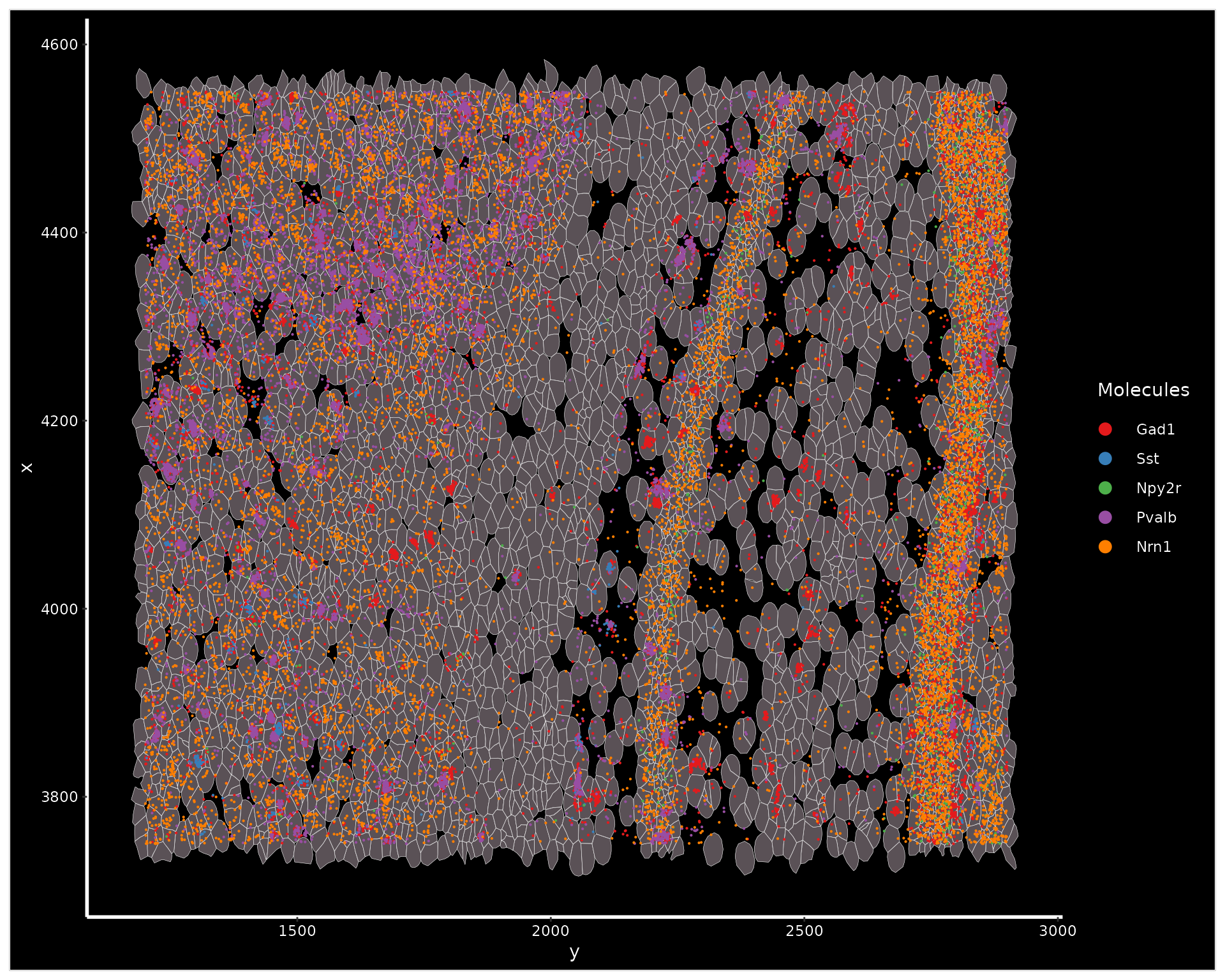
Next, we use SCTransform for normalization followed by standard dimensionality reduction and clustering. This step takes about 5 minutes from start to finish.
xenium.obj <- SCTransform(xenium.obj, assay = "Xenium")
xenium.obj <- RunPCA(xenium.obj, npcs = 30, features = rownames(xenium.obj))
xenium.obj <- RunUMAP(xenium.obj, dims = 1:30)
xenium.obj <- FindNeighbors(xenium.obj, reduction = "pca", dims = 1:30)
xenium.obj <- FindClusters(xenium.obj, resolution = 0.3)
We can then visualize the results of the clustering by coloring each
cell according to its cluster either in UMAP space with
DimPlot() or overlaid on the image with
ImageDimPlot().
DimPlot(xenium.obj)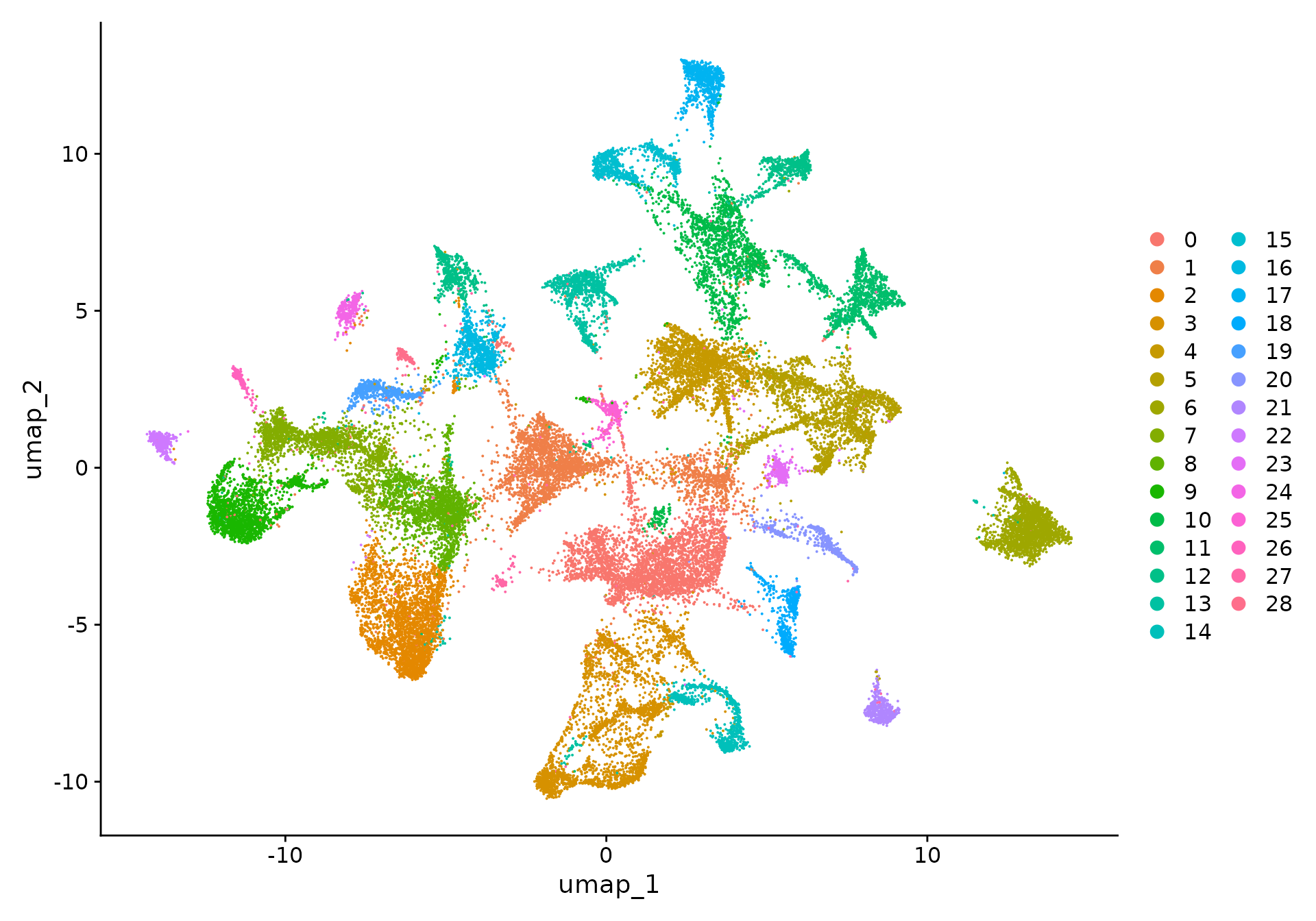
We can visualize the expression level of the markers we looked at earlier on the UMAP coordinates.
FeaturePlot(xenium.obj, features = c("Cux2", "Bcl11b", "Foxp2", "Gad1", "Sst", "Gfap"))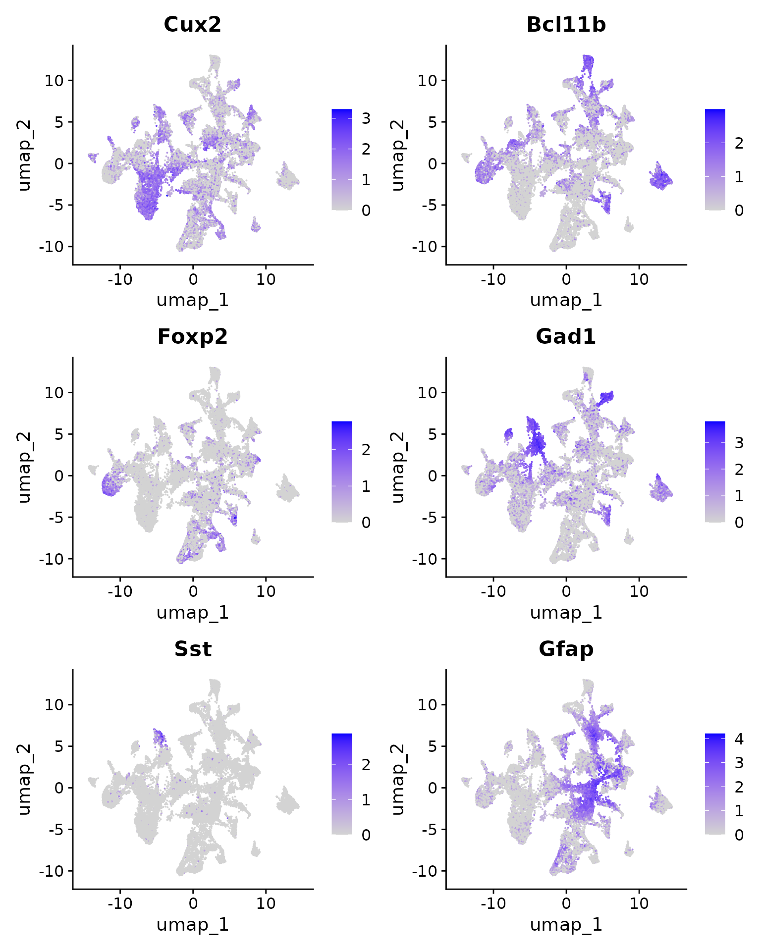
We can now use ImageDimPlot() to color the cell
positions colored by the cluster labels determined in the previous
step.
ImageDimPlot(xenium.obj, cols = "polychrome", size = 0.75)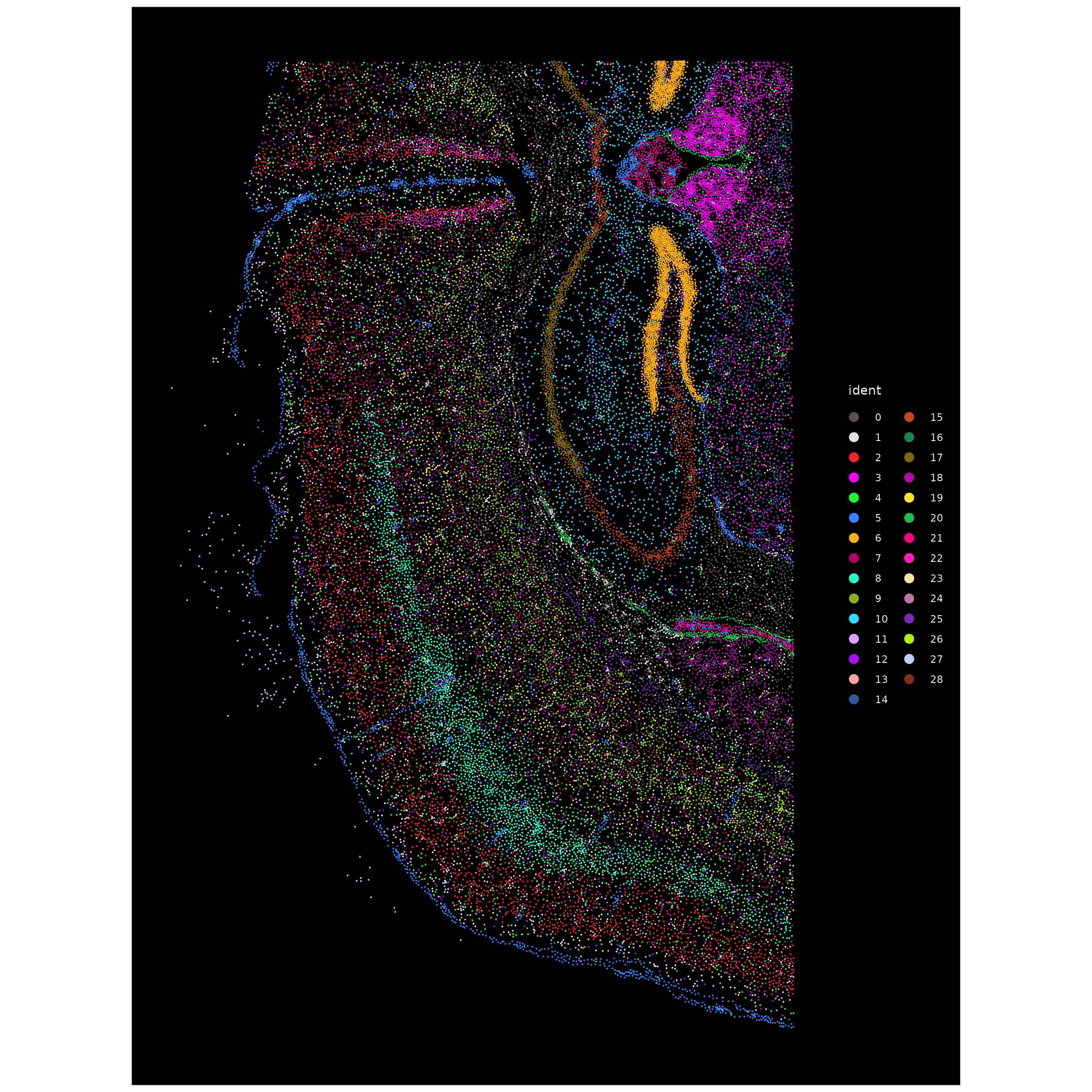
Using the positional information of each cell, we compute spatial niches. We use a cortex reference from the the Allen Brain Institute to annotate cells, so we first crop the dataset to the cortex. The Allen Brain reference can be installed here.
Below, we use Slc17a7 expression to help determine the cortical region.
xenium.obj <- LoadXenium("/brahms/hartmana/vignette_data/xenium_tiny_subset")
p1 <- ImageFeaturePlot(xenium.obj, features = "Slc17a7", axes = TRUE, max.cutoff = "q90")
p1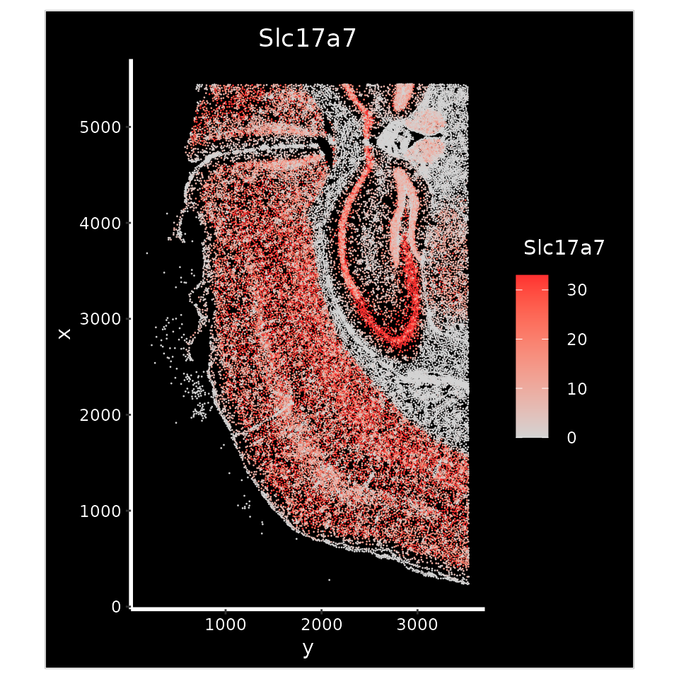
crop <- Crop(xenium.obj[["fov"]], x = c(600, 2100), y = c(900, 4700))
xenium.obj[["crop"]] <- crop
p2 <- ImageFeaturePlot(xenium.obj, fov = "crop", features = "Slc17a7", size = 1, axes = TRUE, max.cutoff = "q90")
p2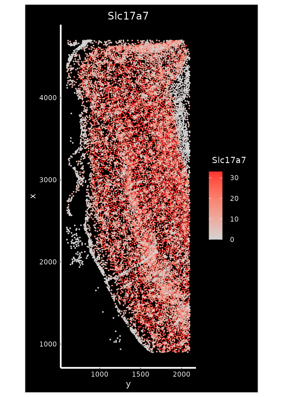
While FindTransferAnchors can be used to integrate
spot-level data from spatial transcriptomic datasets, Seurat v5 also
includes support for the Robust Cell
Type Decomposition, a computational approach to deconvolve
spot-level data from spatial datasets, when provided with an scRNA-seq
reference. RCTD has been shown to accurately annotate spatial data from
a variety of technologies, including SLIDE-seq, Visium, and the 10x
Xenium in-situ spatial platform.
To run RCTD, we first install the spacexr package from
GitHub which implements RCTD.
devtools::install_github("dmcable/spacexr", build_vignettes = FALSE)Counts, cluster, and spot information is extracted from the Seurat
query and reference objects to construct Reference and
SpatialRNA objects used by RCTD for annotation. The output
of the annotation is then added to the Seurat object.
library(spacexr)

query.counts <- GetAssayData(xenium.obj, assay = "Xenium", layer = "counts")[, Cells(xenium.obj[["crop"]])]
coords <- GetTissueCoordinates(xenium.obj[["crop"]], which = "centroids")
rownames(coords) <- coords$cell
coords$cell <- NULL
query <- SpatialRNA(coords, query.counts, colSums(query.counts))
# allen.corted.ref can be downloaded here:
# https://www.dropbox.com/s/cuowvm4vrf65pvq/allen_cortex.rds?dl=1
allen.cortex.ref <- readRDS("/brahms/shared/vignette-data/allen_cortex.rds")
allen.cortex.ref <- UpdateSeuratObject(allen.cortex.ref)

Idents(allen.cortex.ref) <- "subclass"
# remove CR cells because there aren't enough of them for annotation
allen.cortex.ref <- subset(allen.cortex.ref, subset = subclass != "CR")
counts <- GetAssayData(allen.cortex.ref, assay = "RNA", layer = "counts")
cluster <- as.factor(allen.cortex.ref$subclass)
names(cluster) <- colnames(allen.cortex.ref)
nUMI <- allen.cortex.ref$nCount_RNA
names(nUMI) <- colnames(allen.cortex.ref)
nUMI <- colSums(counts)
levels(cluster) <- gsub("/", "-", levels(cluster))
reference <- Reference(counts, cluster, nUMI)
# run RCTD with many cores
RCTD <- create.RCTD(query, reference, max_cores = 8)
RCTD <- run.RCTD(RCTD, doublet_mode = "doublet")
annotations.df <- RCTD@results$results_df
annotations <- annotations.df$first_type
names(annotations) <- rownames(annotations.df)
xenium.obj$predicted.celltype <- annotations
keep.cells <- Cells(xenium.obj)[!is.na(xenium.obj$predicted.celltype)]
xenium.obj <- subset(xenium.obj, cells = keep.cells)
While the previous analyses consider each cell independently, spatial
data enables cells to be defined not just by their neighborhood, but
also by their broader spatial context. In Seurat v5, we introduce
support for ‘niche’ analysis of spatial data, which demarcates regions
of tissue (‘niches’), each of which is defined by a different
composition of spatially adjacent cell types. Inspired by methods in Goltsev
et al, Cell 2018 and He et al, NBT
2022, we consider the ‘local neighborhood’ for each cell -
consisting of its k.neighbor spatially closest neighbors,
and count the occurrences of each cell type present in this
neighborhood. We then use k-means clustering to group cells that have
similar neighborhoods together, into spatial niches.
We call the BuildNicheAssay function from within Seurat
to construct a new assay called niche containing the cell
type composition spatially neighboring each cell. A metadata column
called niches is also returned, which contains cluster
assignments based on the niche assay.
xenium.obj <- BuildNicheAssay(object = xenium.obj, fov = "crop", group.by = "predicted.celltype",
    niches.k = 5, neighbors.k = 30)
We can then group cells either by their cell type identity, or their niche identity. The niches identified clearly demarcate the neuronal layers in the cortex.
celltype.plot <- ImageDimPlot(xenium.obj, group.by = "predicted.celltype", size = 1.5, cols = "polychrome",
    dark.background = F) + ggtitle("Cell type")
niche.plot <- ImageDimPlot(xenium.obj, group.by = "niches", size = 1.5, dark.background = F) + ggtitle("Niches") +
    scale_fill_manual(values = c("#442288", "#6CA2EA", "#B5D33D", "#FED23F", "#EB7D5B"))
celltype.plot | niche.plot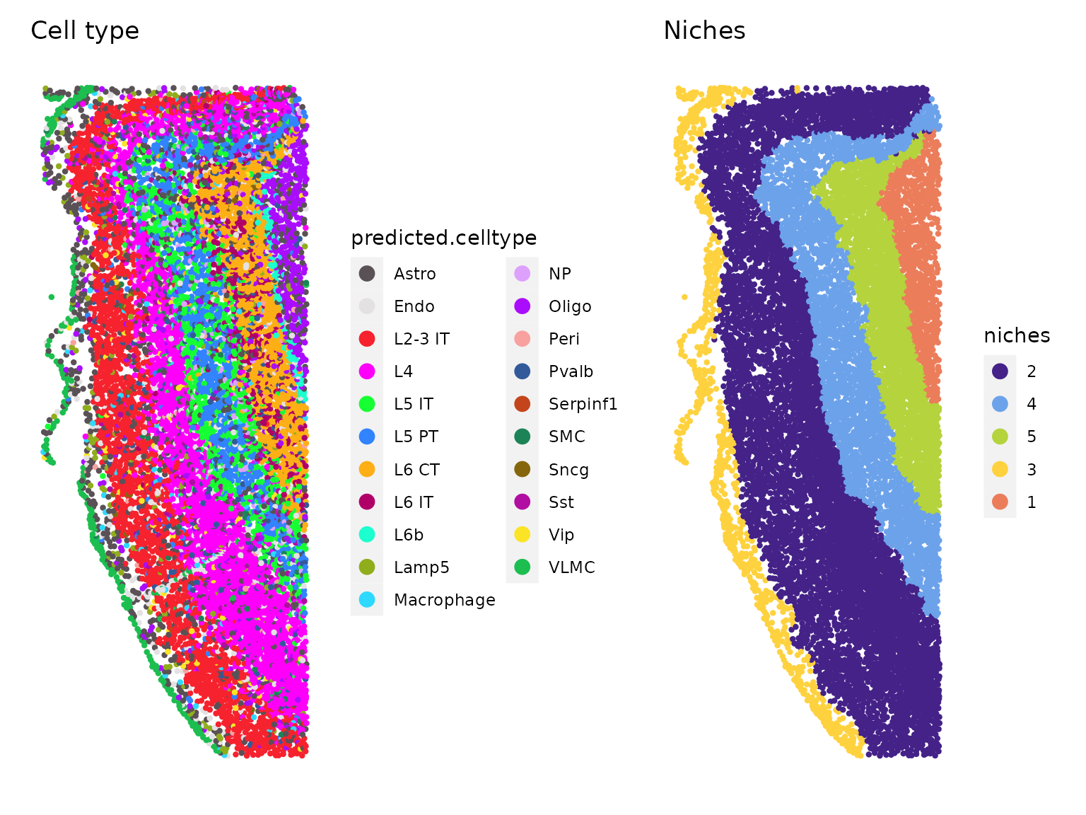
Further, we observe that the composition of each niche is enriched for distinct cell types.
table(xenium.obj$predicted.celltype, xenium.obj$niches)##
## 1 2 3 4 5
## Astro 115 484 241 146 89
## Endo 27 250 66 62 45
## L2-3 IT 0 1749 14 5 6
## L4 2 2163 3 94 14
## L5 IT 2 66 2 627 84
## L5 PT 2 92 4 711 21
## L6 CT 82 2 0 34 857
## L6 IT 4 22 1 56 275
## L6b 95 0 0 2 2
## Lamp5 4 77 61 8 7
## Macrophage 7 48 15 16 10
## Meis2 0 0 0 0 0
## NP 0 1 0 78 9
## Oligo 305 130 42 76 70
## Peri 6 40 4 10 12
## Pvalb 5 155 0 75 54
## Serpinf1 0 5 0 1 1
## SMC 2 34 2 12 2
## Sncg 3 15 1 0 5
## Sst 0 53 0 55 26
## Vip 3 85 5 14 4
## VLMC 2 31 257 7 2Human Lung: Nanostring CosMx Spatial Molecular Imager
This dataset was produced using Nanostring CosMx Spatial Molecular Imager (SMI). The CosMX SMI performs multiplexed single molecule profiling, can profile both RNA and protein targets, and can be applied directly to FFPE tissues. The dataset represents 8 FFPE samples taken from 5 non-small-cell lung cancer (NSCLC) tissues, and is available for public download. The gene panel consists of 960 transcripts.
In this vignette, we load one of 8 samples (lung 5, replicate 1). We
use the LoadNanostring() function, which parses the outputs
available on the public download site. Note that the coordinates for the
cell boundaries were provided by Nanostring by request, and are
available for download here.
For this dataset, instead of performing unsupervised analysis, we map the Nanostring profiles to our Azimuth Healthy Human Lung reference, which was defined by scRNA-seq. We used Azimuth version 0.4.3 with the human lung reference version 1.0.0. You can download the precomputed results here, which include annotations, prediction scores, and a UMAP visualization. The median number of detected transcripts/cell is 249, which does create uncertainty for the annotation process.
nano.obj <- LoadNanostring(data.dir = "/brahms/hartmana/vignette_data/nanostring/lung5_rep1", fov = "lung5.rep1")
# add in precomputed Azimuth annotations
azimuth.data <- readRDS("/brahms/hartmana/vignette_data/nanostring_data.Rds")
nano.obj <- AddMetaData(nano.obj, metadata = azimuth.data$annotations)
nano.obj[["proj.umap"]] <- azimuth.data$umap
Idents(nano.obj) <- nano.obj$predicted.annotation.l1

nano.obj <- SCTransform(nano.obj, assay = "Nanostring", clip.range = c(-10, 10), verbose = FALSE)

# text display of annotations and prediction scores
head(slot(object = nano.obj, name = "meta.data")[2:5])
## nCount_Nanostring nFeature_Nanostring predicted.annotation.l1
## 1_1 23 19 Dendritic
## 2_1 26 23 Macrophage
## 3_1 74 51 Neuroendocrine
## 4_1 60 48 Macrophage
## 5_1 52 39 Macrophage
## 6_1 5 5 CD4 T
## predicted.annotation.l1.score
## 1_1 0.5884506
## 2_1 0.5707920
## 3_1 0.5449661
## 4_1 0.6951970
## 5_1 0.8155319
## 6_1 0.5677324We can visualize the Nanostring cells and annotations, projected onto the reference-defined UMAP. Note that for this NSCLC sample, tumor samples are annotated as ‘basal’, which is the closest cell type match in the healthy reference.
DimPlot(nano.obj)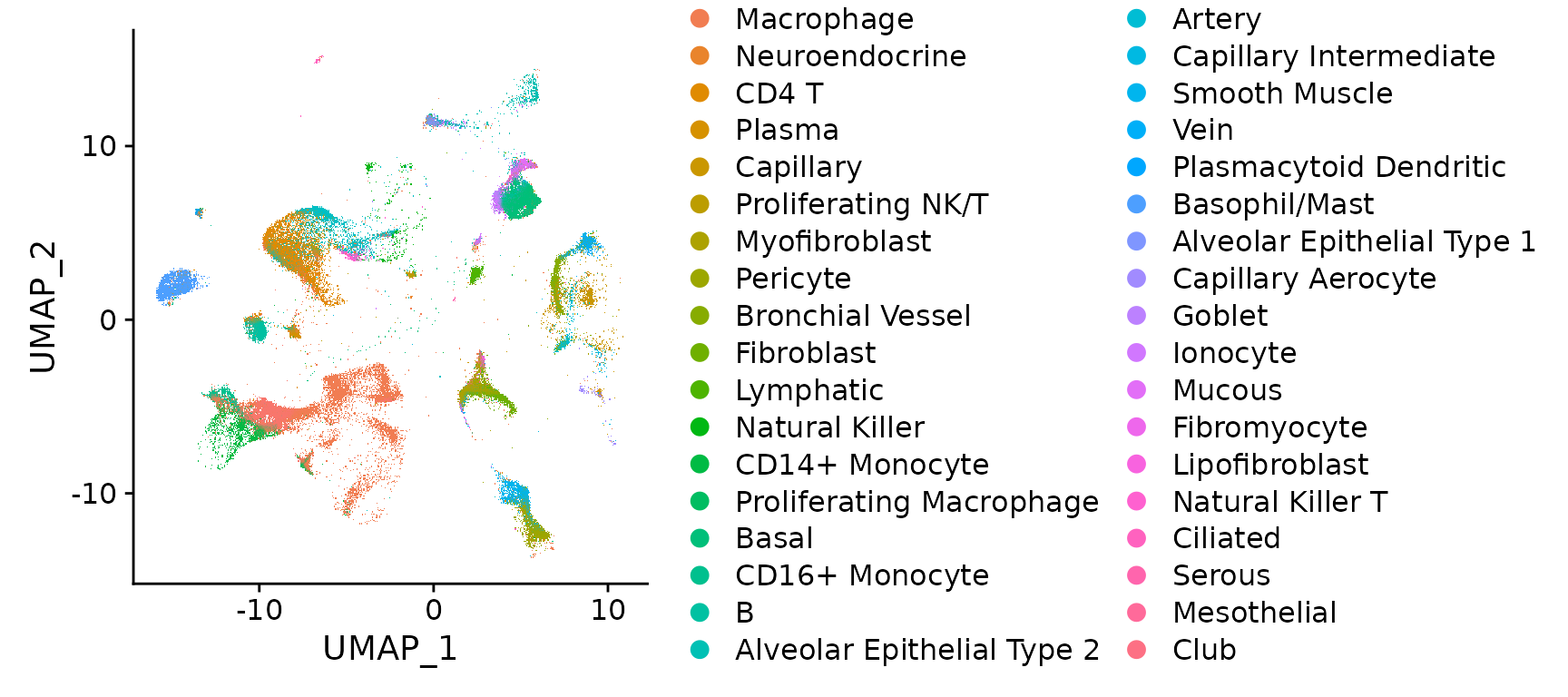
Visualization of cell type and expression localization patterns
As in the previous example, ImageDimPlot() plots c ells
based on their spatial locations, and colors them based on their
assigned cell type. Notice that the basal cell population (tumor cells)
is tightly spatially organized, as expected.
ImageDimPlot(nano.obj, fov = "lung5.rep1", axes = TRUE, cols = "glasbey")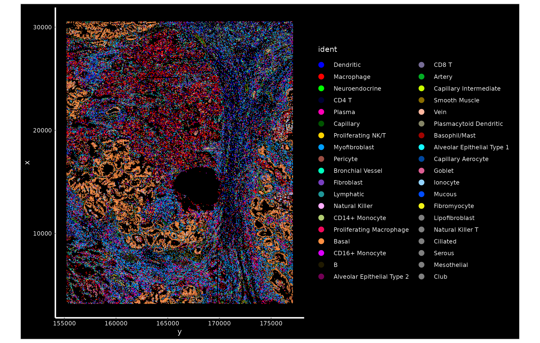
Since there are many cell types present, we can highlight the localization of a few select groups.
ImageDimPlot(nano.obj, fov = "lung5.rep1", cells = WhichCells(nano.obj, idents = c("Basal", "Macrophage",
    "Smooth Muscle", "CD4 T")), cols = c("red", "green", "blue", "orange"), size = 0.6)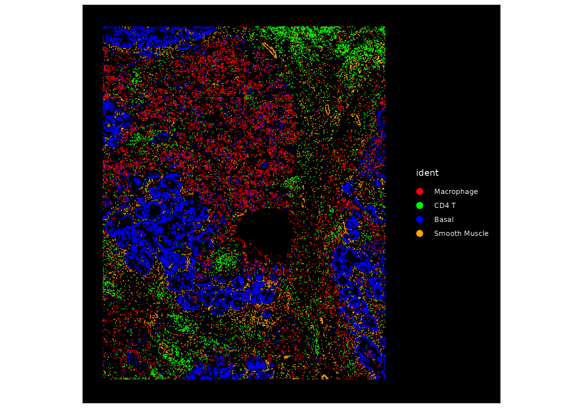
We can also visualize gene expression markers a few different ways:
VlnPlot(nano.obj, features = "KRT17", assay = "Nanostring", layer = "counts", pt.size = 0.1, y.max = 30) +
    NoLegend()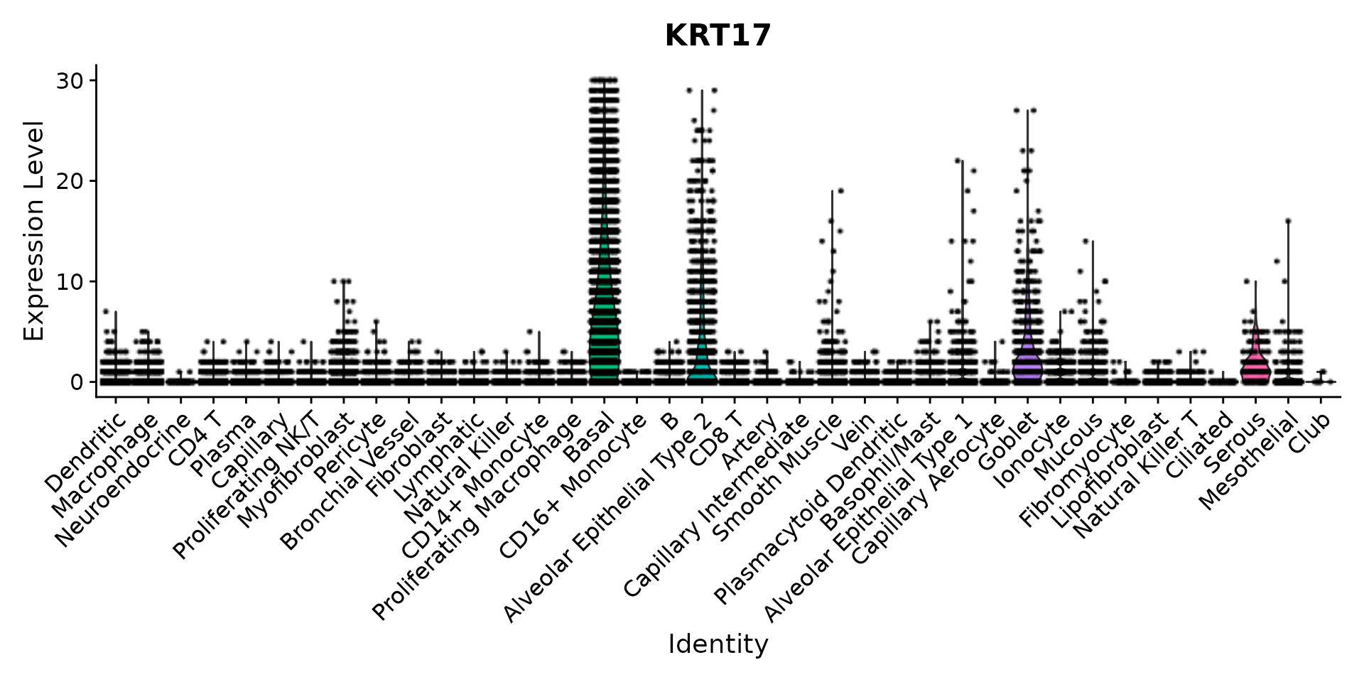
FeaturePlot(nano.obj, features = "KRT17", max.cutoff = "q95")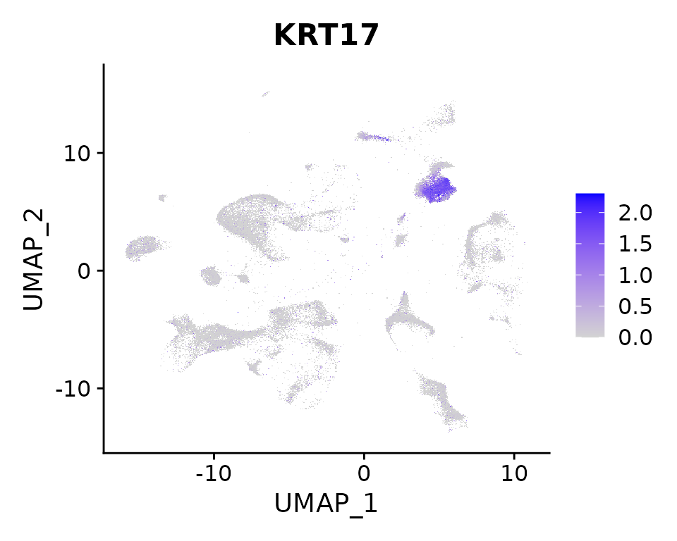
p1 <- ImageFeaturePlot(nano.obj, fov = "lung5.rep1", features = "KRT17", max.cutoff = "q95")
p2 <- ImageDimPlot(nano.obj, fov = "lung5.rep1", alpha = 0.3, molecules = "KRT17", nmols = 10000) +
    NoLegend()
p1 + p2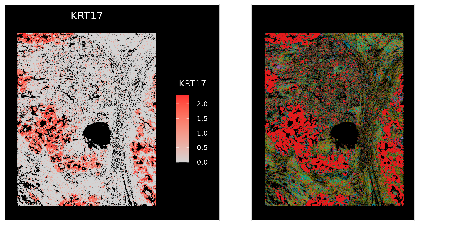
We can plot molecules in order to co-visualize the expression of multiple markers, including KRT17 (basal cells), C1QA (macrophages), IL7R (T cells), and TAGLN (Smooth muscle cells).
# Plot some of the molecules which seem to display spatial correlation with each other
ImageDimPlot(nano.obj, fov = "lung5.rep1", group.by = NA, alpha = 0.3, molecules = c("KRT17", "C1QA",
    "IL7R", "TAGLN"), nmols = 20000)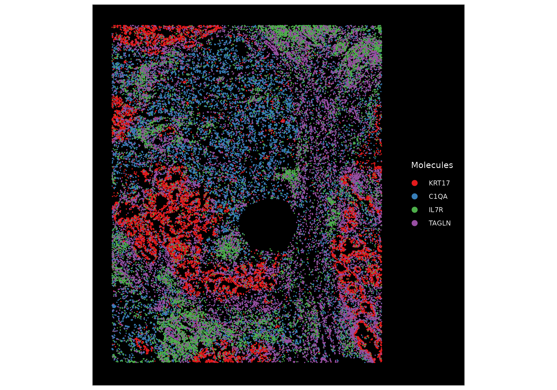
We zoom in on one basal-rich region using the Crop()
function. Once zoomed-in, we can visualize individual cell boundaries as
well in all visualizations.
basal.crop <- Crop(nano.obj[["lung5.rep1"]], x = c(159500, 164000), y = c(8700, 10500))
nano.obj[["zoom1"]] <- basal.crop
DefaultBoundary(nano.obj[["zoom1"]]) <- "segmentation"
ImageDimPlot(nano.obj, fov = "zoom1", cols = "polychrome", coord.fixed = FALSE)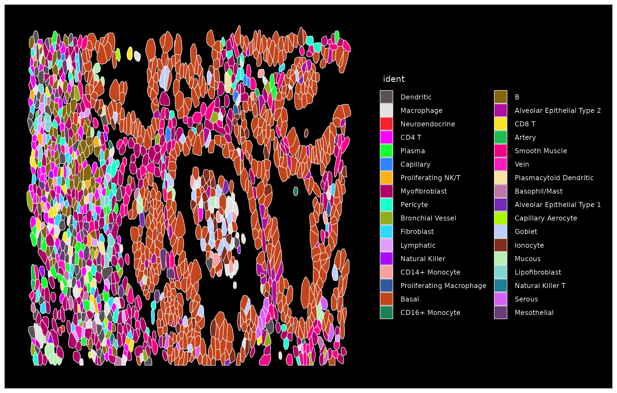
# note the clouds of TPSAB1 molecules denoting mast cells
ImageDimPlot(nano.obj, fov = "zoom1", cols = "polychrome", alpha = 0.3, molecules = c("KRT17", "IL7R",
    "TPSAB1"), mols.size = 0.3, nmols = 20000, border.color = "black", coord.fixed = FALSE)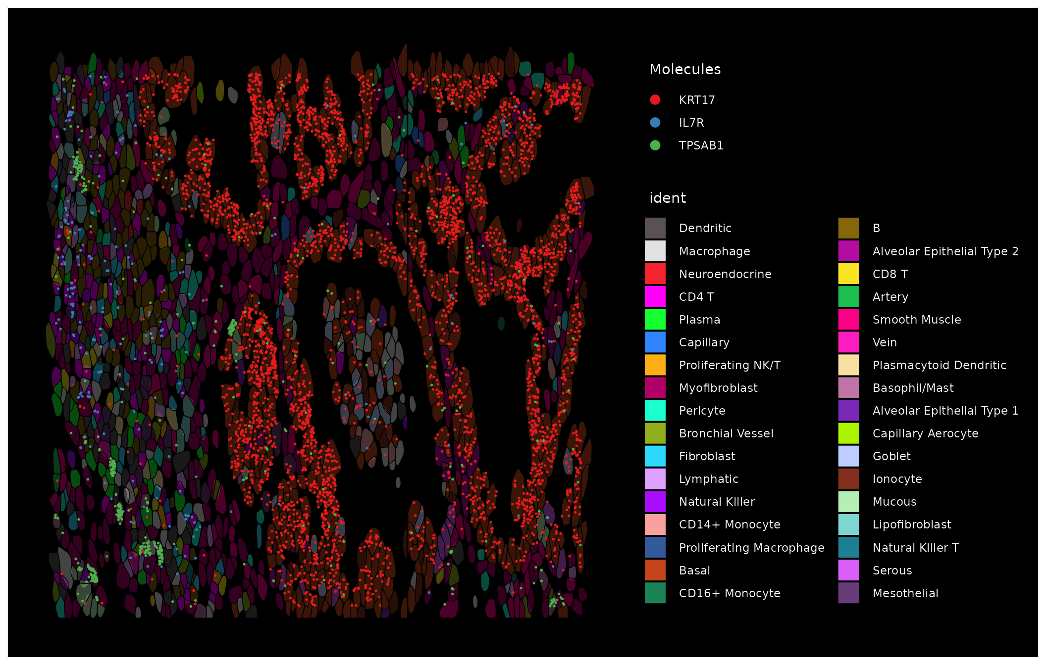
Human Lymph Node: Akoya CODEX system
This dataset was produced using Akoya CODEX system. The CODEX system performs multiplexed spatially-resolved protein profiling, iteratively visualizing antibody-binding events. The dataset here represents a tissue section from a human lymph node, and was generated by the University of Florida as part of the Human Biomolecular Atlas Program (HuBMAP). More information about the sample and experiment is available here. The protein panel in this dataset consists of 28 markers, and protein intensities were quantified as part of the Akoya processor pipeline, which outputs a CSV file providing the intensity of each marker in each cell, as well as the cell coordinates. The file is available for public download via Globus here.
First, we load in the data of a HuBMAP dataset using the
LoadAkoya() function in Seurat:
codex.obj <- LoadAkoya(filename = "/brahms/hartmana/vignette_data/LN7910_20_008_11022020_reg001_compensated.csv",
    type = "processor", fov = "HBM754.WKLP.262")
We can now run unsupervised analysis to identify cell clusters. To normalize the protein data, we use centered log-ratio based normalization, as we typically apply to the protein modality of CITE-seq data. We then run dimensional reduction and graph-based clustering.
codex.obj <- NormalizeData(object = codex.obj, normalization.method = "CLR", margin = 2)
codex.obj <- ScaleData(codex.obj)
VariableFeatures(codex.obj) <- rownames(codex.obj)  # since the panel is small, treat all features as variable.
codex.obj <- RunPCA(object = codex.obj, npcs = 20, verbose = FALSE)
codex.obj <- RunUMAP(object = codex.obj, dims = 1:20, verbose = FALSE)
codex.obj <- FindNeighbors(object = codex.obj, dims = 1:20, verbose = FALSE)
codex.obj <- FindClusters(object = codex.obj, verbose = FALSE, resolution = 0.4, n.start = 1)
We can visualize the cell clusters based on a protein intensity-based UMAP embedding, or also based on their spatial location.
ImageDimPlot(codex.obj, cols = "parade")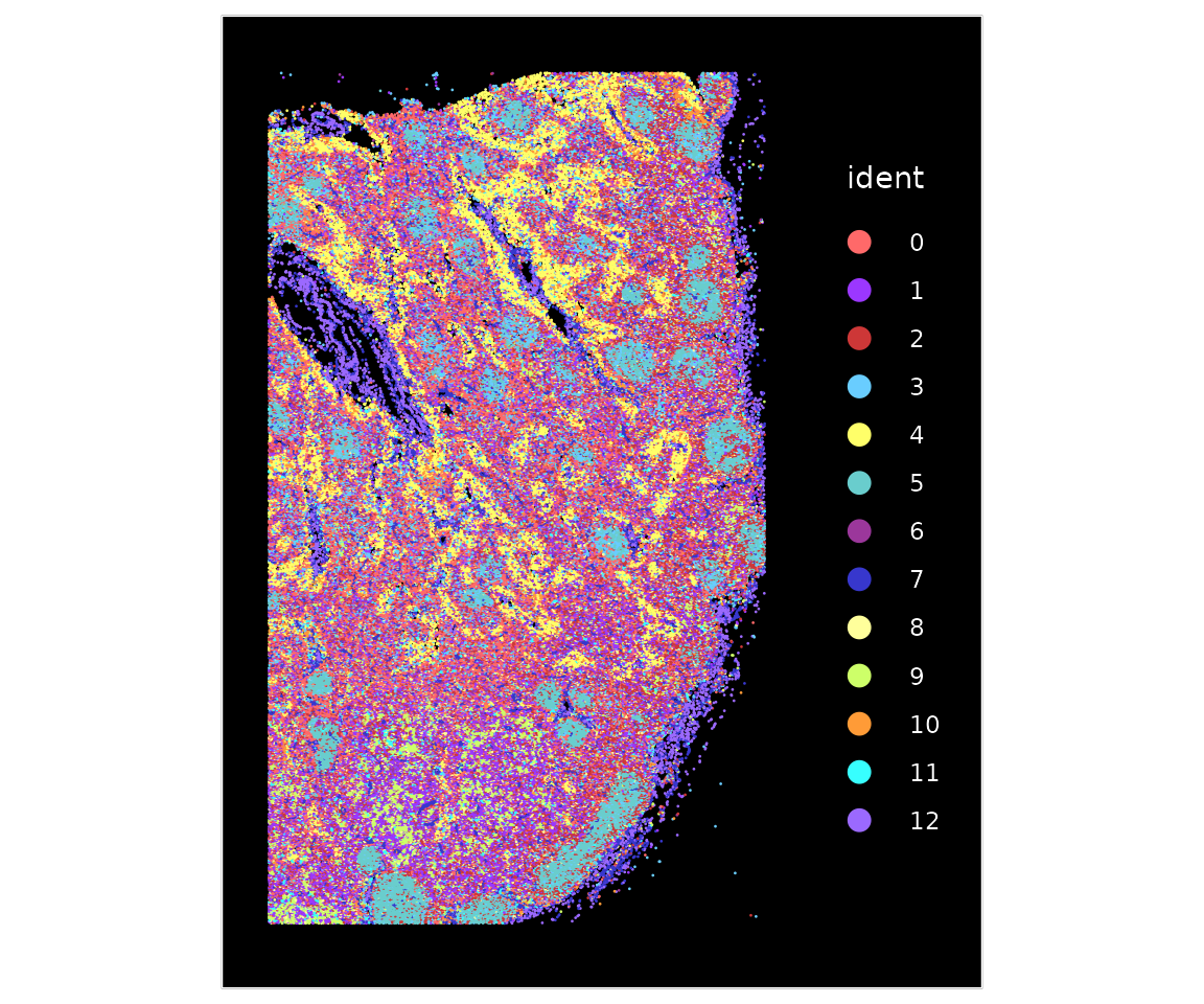
The expression patters of individual markers clearly denote different cell types and spatial structures, including Lyve1 (lymphatic endothelial cells), CD34 (blood endothelial cells), and CD21 (B cells). As expected, endothelial cells group together into vessels, and B cells are key components of specialized microstructures known as germinal zones. You can read more about protein markers in this dataset, as well as cellular networks in human lynmphatic tissues, in this preprint.
p1 <- ImageFeaturePlot(codex.obj, fov = "HBM754.WKLP.262", features = c("CD34", "CD21", "Lyve1"),
    min.cutoff = "q10", max.cutoff = "q90")
p2 <- ImageDimPlot(codex.obj, fov = "HBM754.WKLP.262", cols = "parade")
p1 + p2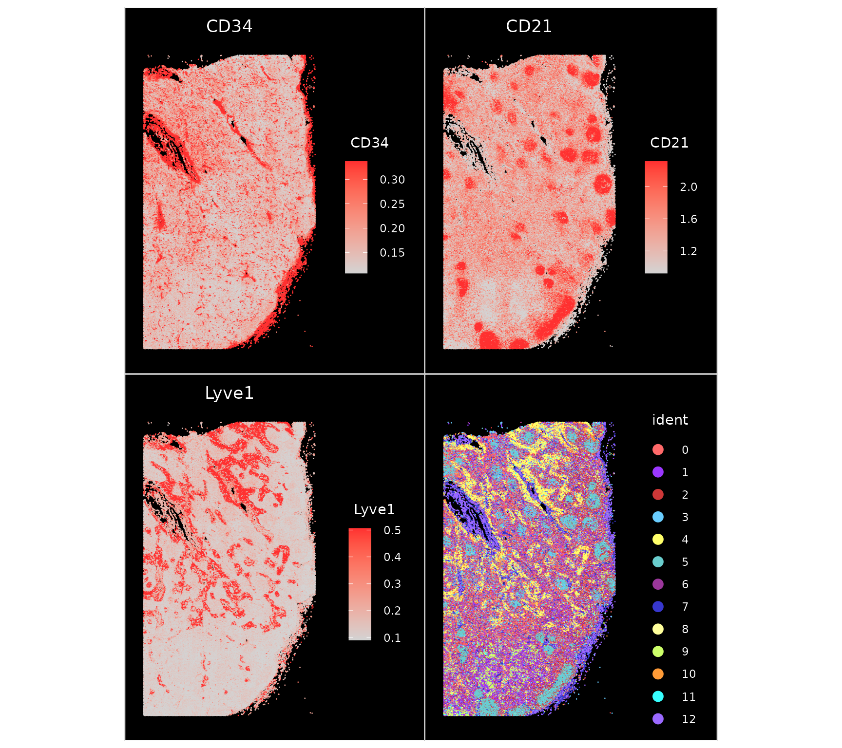
Each of these datasets represents an opportunity to learn organizing principles that govern the spatial localization of different cell types. Stay tuned for future updates to Seurat enabling further exploration and characterization of the relationship between spatial position and molecular state.
Session Info
## R version 4.5.2 (2025-10-31)
## Platform: x86_64-pc-linux-gnu
## Running under: Ubuntu 24.04.4 LTS
##
## Matrix products: default
## BLAS:   /usr/lib/x86_64-linux-gnu/openblas-pthread/libblas.so.3
## LAPACK: /usr/lib/x86_64-linux-gnu/openblas-pthread/libopenblasp-r0.3.26.so;  LAPACK version 3.12.0
##
## locale:
##  [1] LC_CTYPE=en_US.UTF-8       LC_NUMERIC=C
##  [3] LC_TIME=en_US.UTF-8        LC_COLLATE=en_US.UTF-8
##  [5] LC_MONETARY=en_US.UTF-8    LC_MESSAGES=en_US.UTF-8
##  [7] LC_PAPER=en_US.UTF-8       LC_NAME=C
##  [9] LC_ADDRESS=C               LC_TELEPHONE=C
## [11] LC_MEASUREMENT=en_US.UTF-8 LC_IDENTIFICATION=C
##
## time zone: Etc/UTC
## tzcode source: system (glibc)
##
## attached base packages:
## [1] stats     graphics  grDevices utils     datasets  methods   base
##
## other attached packages:
## [1] spacexr_2.2.1      ggplot2_4.0.3      future_1.70.0      Seurat_5.5.0
## [5] SeuratObject_5.4.0 sp_2.2-1
##
## loaded via a namespace (and not attached):
##   [1] RcppAnnoy_0.0.23            splines_4.5.2
##   [3] later_1.4.8                 tibble_3.3.1
##   [5] R.oo_1.27.1                 polyclip_1.10-7
##   [7] fastDummies_1.7.6           lifecycle_1.0.5
##   [9] sf_1.1-0                    doParallel_1.0.17
##  [11] globals_0.19.1              lattice_0.22-7
##  [13] hdf5r_1.3.12                MASS_7.3-65
##  [15] magrittr_2.0.5              limma_3.66.0
##  [17] plotly_4.12.0               sass_0.4.10
##  [19] rmarkdown_2.30              jquerylib_0.1.4
##  [21] yaml_2.3.12                 httpuv_1.6.16
##  [23] otel_0.2.0                  glmGamPoi_1.22.0
##  [25] sctransform_0.4.3           spam_2.11-3
##  [27] spatstat.sparse_3.1-0       reticulate_1.46.0
##  [29] cowplot_1.2.0               pbapply_1.7-4
##  [31] DBI_1.3.0                   RColorBrewer_1.1-3
##  [33] abind_1.4-8                 Rtsne_0.17
##  [35] GenomicRanges_1.62.1        purrr_1.2.1
##  [37] presto_1.0.0                R.utils_2.13.0
##  [39] BiocGenerics_0.56.0         IRanges_2.44.0
##  [41] S4Vectors_0.48.1            ggrepel_0.9.8
##  [43] irlba_2.3.7                 listenv_0.10.1
##  [45] spatstat.utils_3.2-2        units_1.0-1
##  [47] goftest_1.2-3               RSpectra_0.16-2
##  [49] spatstat.random_3.4-5       fitdistrplus_1.2-6
##  [51] parallelly_1.47.0           pkgdown_2.2.0
##  [53] codetools_0.2-20            DelayedArray_0.36.1
##  [55] tidyselect_1.2.1            farver_2.1.2
##  [57] matrixStats_1.5.0           stats4_4.5.2
##  [59] spatstat.explore_3.8-0      Seqinfo_1.0.0
##  [61] jsonlite_2.0.0              e1071_1.7-17
##  [63] progressr_0.19.0            iterators_1.0.14
##  [65] ggridges_0.5.7              survival_3.8-3
##  [67] systemfonts_1.3.2           foreach_1.5.2
##  [69] tools_4.5.2                 ragg_1.5.1
##  [71] ica_1.0-3                   Rcpp_1.1.1-1.1
##  [73] glue_1.8.0                  gridExtra_2.3
##  [75] SparseArray_1.10.10         xfun_0.56
##  [77] MatrixGenerics_1.22.0       dplyr_1.2.0
##  [79] withr_3.0.2                 formatR_1.14
##  [81] fastmap_1.2.0               digest_0.6.39
##  [83] R6_2.6.1                    mime_0.13
##  [85] textshaping_1.0.5           Cairo_1.7-0
##  [87] scattermore_1.2             tensor_1.5.1
##  [89] dichromat_2.0-0.1           spatstat.data_3.1-9
##  [91] R.methodsS3_1.8.2           tidyr_1.3.2
##  [93] generics_0.1.4              data.table_1.18.2.1
##  [95] class_7.3-23                httr_1.4.8
##  [97] htmlwidgets_1.6.4           S4Arrays_1.10.1
##  [99] uwot_0.2.4                  pkgconfig_2.0.3
## [101] gtable_0.3.6                lmtest_0.9-40
## [103] S7_0.2.1                    XVector_0.50.0
## [105] htmltools_0.5.9             dotCall64_1.2
## [107] scales_1.4.0                Biobase_2.70.0
## [109] png_0.1-9                   spatstat.univar_3.1-7
## [111] knitr_1.51                  reshape2_1.4.5
## [113] nlme_3.1-168                proxy_0.4-29
## [115] cachem_1.1.0                zoo_1.8-15
## [117] stringr_1.6.0               KernSmooth_2.23-26
## [119] vipor_0.4.7                 parallel_4.5.2
## [121] miniUI_0.1.2                arrow_23.0.1.2
## [123] ggrastr_1.0.2               desc_1.4.3
## [125] pillar_1.11.1               grid_4.5.2
## [127] vctrs_0.7.1                 RANN_2.6.2
## [129] promises_1.5.0              beachmat_2.26.0
## [131] xtable_1.8-8                cluster_2.1.8.2
## [133] beeswarm_0.4.0              evaluate_1.0.5
## [135] cli_3.6.6                   compiler_4.5.2
## [137] rlang_1.2.0                 future.apply_1.20.2
## [139] labeling_0.4.3              classInt_0.4-11
## [141] ggbeeswarm_0.7.3            plyr_1.8.9
## [143] fs_2.1.0                    stringi_1.8.7
## [145] viridisLite_0.4.3           deldir_2.0-4
## [147] assertthat_0.2.1            lazyeval_0.2.3
## [149] spatstat.geom_3.7-3         Matrix_1.7-5
## [151] RcppHNSW_0.6.0              patchwork_1.3.2
## [153] bit64_4.6.0-1               statmod_1.5.1
## [155] shiny_1.13.0                SummarizedExperiment_1.40.0
## [157] ROCR_1.0-12                 igraph_2.3.0
## [159] bslib_0.10.0                bit_4.6.0