Sketch-based analysis in Seurat v5

Intro: Sketch-based analysis in Seurat v5

As single-cell sequencing technologies continue to improve in scalability in throughput, the generation of datasets spanning a million or more cells is becoming increasingly routine. In Seurat v5, we introduce new infrastructure and methods to analyze, interpret, and explore these exciting datasets.

In this vignette, we introduce a sketch-based analysis workflow to analyze a 1.3 million cell dataset of the developing mouse brain, freely available from 10x Genomics. Analyzing datasets of this size with standard workflows can be challenging, slow, and memory-intensive. Here we introduce an alternative workflow that is highly scalable, even to datasets ranging beyond 10 million cells in size. Our ‘sketch-based’ workflow involves three new features in Seurat v5:

Infrastructure for on-disk storage of large single-cell datasets

Storing expression matrices in memory can be challenging for extremely large scRNA-seq datasets. In Seurat v5, we introduce support for multiple on-disk storage formats.

‘Sketching’ methods to subsample cells from large datasets while preserving rare populations

As introduced in Hie et al, 2019, cell sketching methods aim to compactly summarize large single-cell datasets in a small number of cells, while preserving the presence of both abundant and rare cell types. In Seurat v5, we leverage this idea to select subsamples (‘sketches’) of cells from large datasets that are stored on-disk. However, after sketching, the subsampled cells can be stored in-memory, allowing for interactive and rapid visualization and exploration. We store sketched cells (in-memory) and the full dataset (on-disk) as two assays in the same Seurat object. Users can then easily switch between the two versions, providing the flexibility to perform quick analyses on a subset of cells in-memory, while retaining access to the full dataset on-disk.

Support for ‘bit-packing’ compression and infrastructure

We demonstrate the on-disk capabilities in Seurat v5 using the BPCells package developed by Ben Parks in the Greenleaf Lab. This package utilizes bit-packing compression and optimized, streaming-compatible C++ code to substantially improve I/O and computational performance when working with on-disk data. To run this vignette please install Seurat v5, using the installation instructions found here. Additionally, you will need to install the BPcells package, using the installation instructions found here.

library(Seurat)
library(BPCells)
library(ggplot2)
# needs to be set for large dataset analysis
options(future.globals.maxSize = 1e9)

Create a Seurat object with a v5 assay for on-disk storage

We start by loading the 1.3M dataset from 10x Genomics using the open_matrix_dir function from BPCells. Note that in our Introduction to on-disk storage vignette, we demonstrate how to create this on-disk representation. This function does not load the dataset into memory, but instead, creates a connection to the data stored on-disk. We then store this on-disk representation in the Seurat object, which is loaded using readRDS as per usual.

# Read the Seurat object, which contains 1.3M cells stored on-disk as part of the 'RNA' assay
obj <- readRDS("/brahms/hartmana/vignette_data/1p3_million_mouse_brain.rds")
obj

## An object of class Seurat 
## 27282 features across 1306127 samples within 1 assay 
## Active assay: RNA (27282 features, 0 variable features)
##  1 layer present: counts

# Note that since the data is stored on-disk, the object size easily fits in-memory (<1GB)
format(object.size(obj), units = "Mb")

## [1] "596.2 Mb"

‘Sketch’ a subset of cells, and load these into memory

We select a subset (‘sketch’) of 50,000 cells (out of 1.3M). Rather than sampling all cells with uniform probability, we compute and sample based off a ‘leverage score’ for each cell, which reflects the magnitude of its contribution to the gene-covariance matrix, and its importance to the overall dataset. In Hao et al, 2022, we demonstrate that the leverage score is highest for rare populations in a dataset. Therefore, our sketched set of 50,000 cells will oversample rare populations, retaining the biological complexity of the sample while drastically compressing the dataset.

The function SketchData takes a normalized single-cell dataset (stored either on-disk or in-memory), and a set of variable features. It returns a Seurat object with a new assay (sketch), consisting of 50,000 cells, but these cells are now stored in-memory. Users can now easily switch between the in-memory and on-disk representation just by changing the default assay.

obj <- NormalizeData(obj)
obj <- FindVariableFeatures(obj)
obj <- SketchData(
  object = obj,
  ncells = 50000,
  method = "LeverageScore",
  sketched.assay = "sketch"
)
obj

## An object of class Seurat 
## 54564 features across 1306127 samples within 2 assays 
## Active assay: sketch (27282 features, 2000 variable features)
##  2 layers present: counts, data
##  1 other assay present: RNA

# switch to analyzing the full dataset (on-disk)
DefaultAssay(obj) <- "RNA"
# switch to analyzing the sketched dataset (in-memory)
DefaultAssay(obj) <- "sketch"

Perform clustering on the sketched dataset

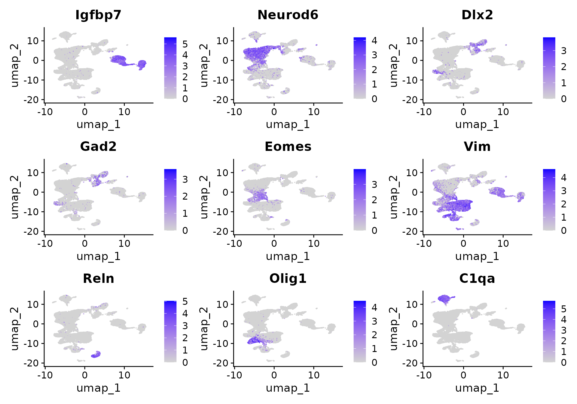
Now that we have compressed the dataset, we can perform standard clustering and visualization of a 50,000 cell dataset. After clustering, we can see groups of cells that clearly correspond to precursors of distinct lineages, including endothelial cells (Igfbp7), Excitatory (Neurod6) and Inhibitory (Dlx2) neurons, Intermediate Progenitors (Eomes), Radial Glia (Vim), Cajal-Retzius cells (Reln), Oligodendroytes (Olig1), and extremely rare populations of macrophages (C1qa) that were oversampled in our sketched data.

DefaultAssay(obj) <- "sketch"
obj <- FindVariableFeatures(obj)
obj <- ScaleData(obj)
obj <- RunPCA(obj)
obj <- FindNeighbors(obj, dims = 1:50)
obj <- FindClusters(obj, resolution = 2)

## Modularity Optimizer version 1.3.0 by Ludo Waltman and Nees Jan van Eck
## 
## Number of nodes: 50000
## Number of edges: 1992657
## 
## Running Louvain algorithm...
## Maximum modularity in 10 random starts: 0.8766
## Number of communities: 51
## Elapsed time: 19 seconds

obj <- RunUMAP(obj, dims = 1:50, return.model = T)
DimPlot(obj, label = T, label.size = 3, reduction = "umap") + NoLegend()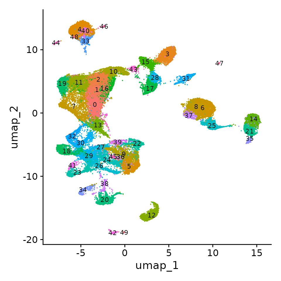

FeaturePlot(
  object = obj,
  features = c(
    "Igfbp7", "Neurod6", "Dlx2", "Gad2",
    "Eomes", "Vim", "Reln", "Olig1", "C1qa"
  ),
  ncol = 3
)

Extend results to the full datasets

We can now extend the cluster labels and dimensional reductions learned on the sketched cells to the full dataset. The ProjectData function projects the on-disk data, onto the sketch assay. It returns a Seurat object that includes a

Dimensional reduction (PCA): The pca.full dimensional reduction extends the pca reduction on the sketched cells to all cells in the dataset
Dimensional reduction (UMAP): The full.umap dimensional reduction extends the umap reduction on the sketched cells to all cells in the dataset
Cluster labels: The cluster_full column in the object metadata now labels all cells in the dataset with one of the cluster labels derived from the sketched cells

obj <- ProjectData(
  object = obj,
  assay = "RNA",
  full.reduction = "pca.full",
  sketched.assay = "sketch",
  sketched.reduction = "pca",
  umap.model = "umap",
  dims = 1:50,
  refdata = list(cluster_full = "seurat_clusters")
)
# now that we have projected the full dataset, switch back to analyzing all cells
DefaultAssay(obj) <- "RNA"

DimPlot(obj, label = T, label.size = 3, reduction = "full.umap", group.by = "cluster_full", alpha = 0.1) + NoLegend()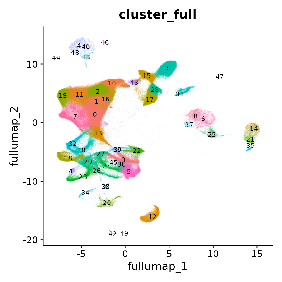

# visualize gene expression on the sketched cells (fast) and the full dataset (slower)
DefaultAssay(obj) <- "sketch"
x1 <- FeaturePlot(obj, "C1qa")
DefaultAssay(obj) <- "RNA"
x2 <- FeaturePlot(obj, "C1qa")
x1 | x2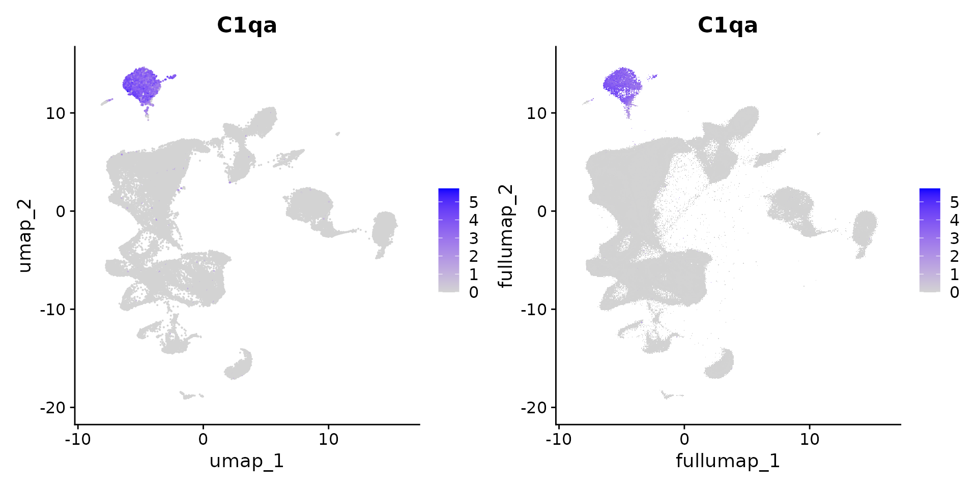

Perform iterative sub-clustering

Now that we have performed an initial analysis of the dataset, we can iteratively ‘zoom-in’ on a cell subtype of interest, extract all cells of this type, and perform iterative sub-clustering. For example, we can see that Dlx2+ interneuron precursors are defined by clusters 2, 15, 18, 28 and 40.

DefaultAssay(obj) <- "sketch"
VlnPlot(obj, "Dlx2")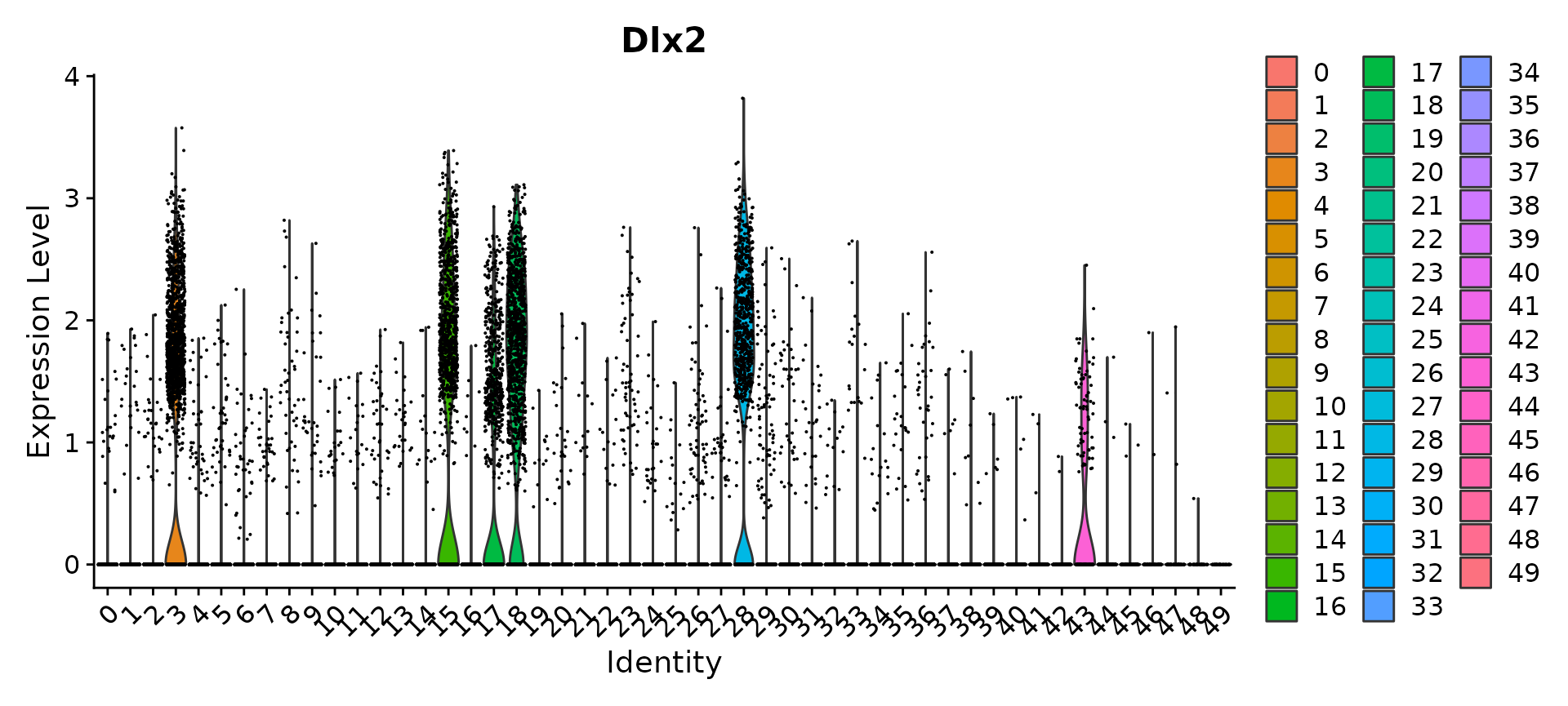

We therefore extract all cells from the full on-disk dataset that are present in these clusters. There are 200,892 of them. Since this is a manageable number, we can convert these data from on-disk storage into in-memory storage. We can then proceed with standard clustering.

# subset cells in these clusters. Note that the data remains on-disk after subsetting
obj.sub <- subset(obj, subset = cluster_full %in% c(2, 15, 18, 28, 40))
DefaultAssay(obj.sub) <- "RNA"

# now convert the RNA assay (previously on-disk) into an in-memory representation (sparse Matrix)
# we only convert the data layer, and keep the counts on-disk
obj.sub[["RNA"]]$data <- as(obj.sub[["RNA"]]$data, Class = "dgCMatrix")

# recluster the cells
obj.sub <- FindVariableFeatures(obj.sub)
obj.sub <- ScaleData(obj.sub)
obj.sub <- RunPCA(obj.sub)
obj.sub <- RunUMAP(obj.sub, dims = 1:30)
obj.sub <- FindNeighbors(obj.sub, dims = 1:30)
obj.sub <- FindClusters(obj.sub)

## Modularity Optimizer version 1.3.0 by Ludo Waltman and Nees Jan van Eck
## 
## Number of nodes: 236276
## Number of edges: 5470656
## 
## Running Louvain algorithm...
## Maximum modularity in 10 random starts: 0.8577
## Number of communities: 28
## Elapsed time: 191 seconds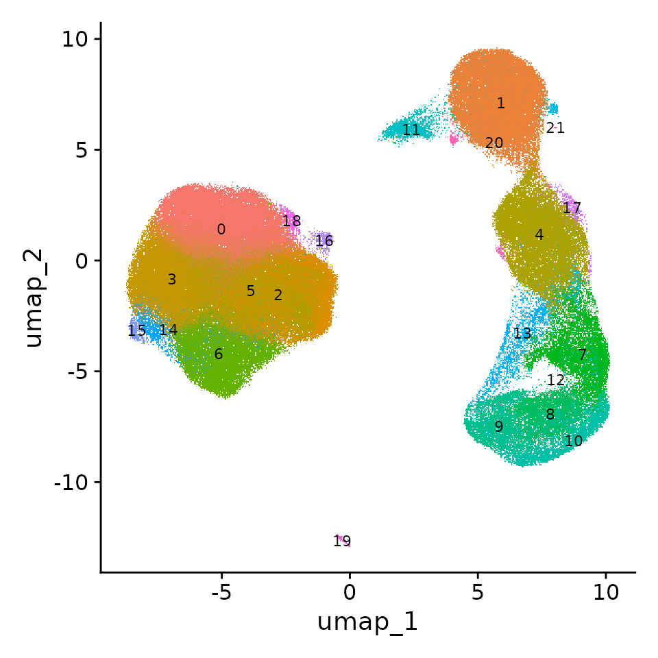

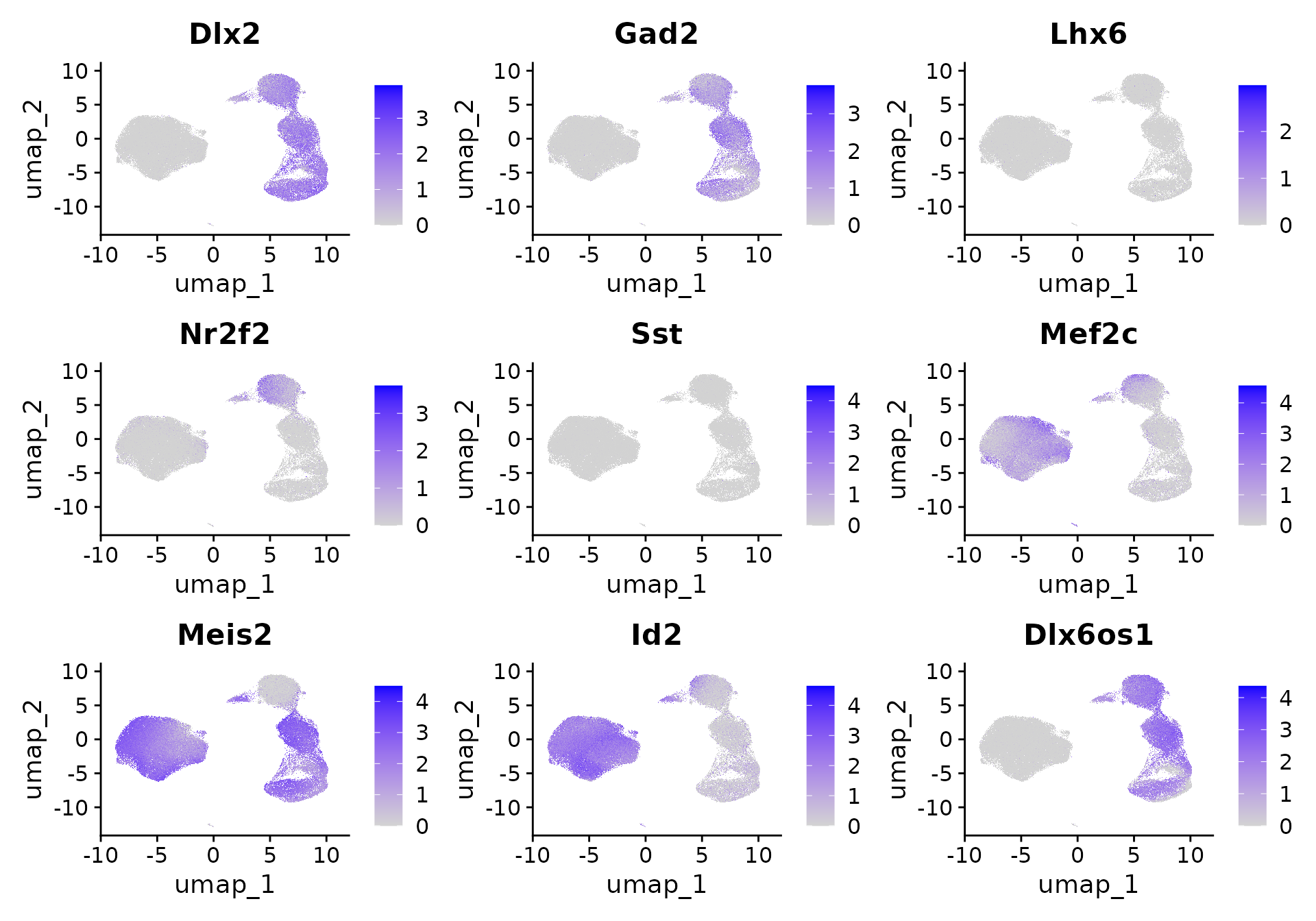
DimPlot(obj.sub, label = T, label.size = 3) + NoLegend()

Note that we can start to see distinct interneuron lineages emerging in this dataset. We can see a clear separation of interneuron precursors that originated from the medial ganglionic eminence (Lhx6) or caudal ganglionic eminence (Nr2f2). We can further see the emergence of Sst (Sst) and Pvalb (Mef2c)-committed interneurons, and a CGE-derived Meis2-expressing progenitor population. These results closely mirror our findings from Mayer, Hafemeister, Bandler* et al, Nature 2018, where we enriched for interneuron precursors using a Dlx6a-cre fate-mapping strategy. Here, we obtain similar results using only computational enrichment, enabled by the large size of the original dataset.

FeaturePlot(
  object = obj.sub,
  features = c(
    "Dlx2", "Gad2", "Lhx6", "Nr2f2", "Sst",
    "Mef2c", "Meis2", "Id2", "Dlx6os1"
  ),
  ncol = 3
)

Session Info

sessionInfo()