Integrative analysis in Seurat v5
Compiled: May 22, 2026
Source:vignettes/seurat5_integration.Rmd
seurat5_integration.Rmd
library(Seurat)
library(SeuratData)
library(SeuratWrappers)
library(Azimuth)
library(ggplot2)
library(patchwork)
options(future.globals.maxSize = 1e+10)
Introduction
Integration of single-cell sequencing datasets, for example across
experimental batches, donors, or conditions, is often an important step
in scRNA-seq workflows. Integrative analysis can help to match shared
cell types and states across datasets, which can boost statistical
power, and most importantly, facilitate accurate comparative analysis
across datasets. In previous versions of Seurat we introduced methods
for integrative analysis, including our ‘anchor-based’ integration
workflow. Many labs have also published powerful and pioneering methods,
including Harmony and scVI, for
integrative analysis. We recognize that while the goal of matching
shared cell types across datasets may be important for many problems,
users may also be concerned about which method to use, or that
integration could result in a loss of biological resolution. In Seurat
v5, we introduce more flexible and streamlined infrastructure to run
different integration algorithms with a single line of code. This makes
it easier to explore the results of different integration methods, and
to compare these results to a workflow that excludes integration steps.
For this vignette, we use a dataset of
human PBMC profiled with seven different technologies, profiled as
part of a systematic comparative analysis (pbmcsca). The
data is available as part of our SeuratData
package.
Layers in the Seurat v5 object
Seurat v5 assays store data in layers. These layers can store raw,
un-normalized counts (layer='counts'), normalized data
(layer='data'), or z-scored/variance-stabilized data
(layer='scale.data'). We can load in the data, remove
low-quality cells, and obtain predicted cell annotations (which will be
useful for assessing integration later), using our Azimuth
pipeline.
# load in the pbmc systematic comparative analysis dataset
obj <- LoadData("pbmcsca")
obj <- subset(obj, nFeature_RNA > 1000)
obj <- RunAzimuth(obj, reference = "pbmcref")
# currently, the object has two layers in the RNA assay: counts, and data
obj
## An object of class Seurat
## 33789 features across 10434 samples within 4 assays
## Active assay: RNA (33694 features, 0 variable features)
## 2 layers present: counts, data
## 3 other assays present: prediction.score.celltype.l1, prediction.score.celltype.l2, prediction.score.celltype.l3
## 2 dimensional reductions calculated: integrated_dr, ref.umapThe object contains data from nine different batches (stored in the
Method column in the object metadata), representing seven
different technologies. We will aim to integrate the different batches
together. In previous versions of Seurat, we would require the data to
be represented as nine different Seurat objects. When using Seurat v5
assays, we can instead keep all the data in one object, but simply split
the layers. After splitting, there are now 18 layers (a
counts and data layer for each batch). We can
also run a standard scRNA-seq analysis (i.e. without integration). Note
that since the data is split into layers, normalization and variable
feature identification is performed for each batch independently (a
consensus set of variable features is automatically identified).
obj[["RNA"]] <- split(obj[["RNA"]], f = obj$Method)
obj
## An object of class Seurat
## 33789 features across 10434 samples within 4 assays
## Active assay: RNA (33694 features, 0 variable features)
## 18 layers present: counts.Smart-seq2, counts.CEL-Seq2, counts.10x_Chromium_v2_A, counts.10x_Chromium_v2_B, counts.10x_Chromium_v3, counts.Drop-seq, counts.Seq-Well, counts.inDrops, counts.10x_Chromium_v2, data.Smart-seq2, data.CEL-Seq2, data.10x_Chromium_v2_A, data.10x_Chromium_v2_B, data.10x_Chromium_v3, data.Drop-seq, data.Seq-Well, data.inDrops, data.10x_Chromium_v2
## 3 other assays present: prediction.score.celltype.l1, prediction.score.celltype.l2, prediction.score.celltype.l3
## 2 dimensional reductions calculated: integrated_dr, ref.umap
obj <- NormalizeData(obj)
obj <- FindVariableFeatures(obj)
obj <- ScaleData(obj)
obj <- RunPCA(obj)
We can now visualize the results of a standard analysis without integration. Note that cells are grouping both by cell type and by underlying method. While a UMAP analysis is just a visualization of this, clustering this dataset would return predominantly batch-specific clusters. Especially if previous cell-type annotations were not available, this would make downstream analysis extremely challenging.
obj <- FindNeighbors(obj, dims = 1:30, reduction = "pca")
obj <- FindClusters(obj, resolution = 2, cluster.name = "unintegrated_clusters")
## Modularity Optimizer version 1.3.0 by Ludo Waltman and Nees Jan van Eck
##
## Number of nodes: 10434
## Number of edges: 412660
##
## Running Louvain algorithm...
## Maximum modularity in 10 random starts: 0.8981
## Number of communities: 48
## Elapsed time: 1 seconds
obj <- RunUMAP(obj, dims = 1:30, reduction = "pca", reduction.name = "umap.unintegrated")
# visualize by batch and cell type annotation cell type annotations were
# previously added by Azimuth
DimPlot(obj, reduction = "umap.unintegrated", group.by = c("Method", "predicted.celltype.l2"))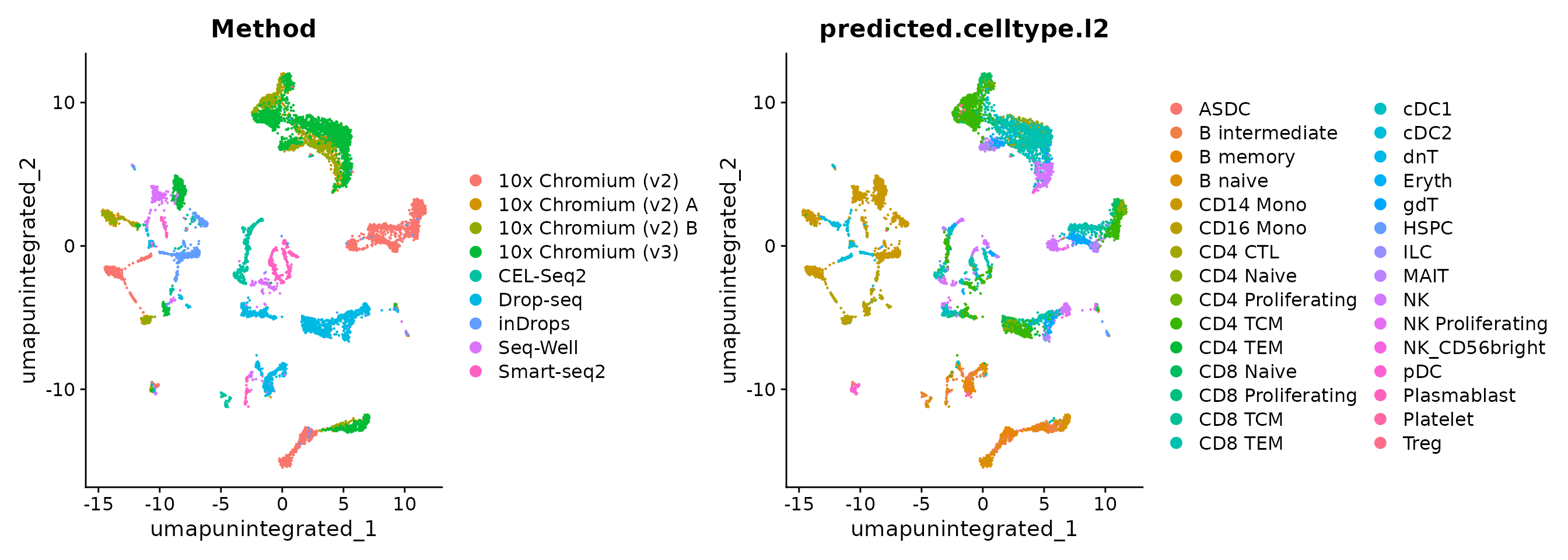
Perform streamlined (one-line) integrative analysis
Seurat v5 enables streamlined integrative analysis using the
IntegrateLayers function. The method currently supports
five integration methods. Each of these methods performs integration in
low-dimensional space, and returns a dimensional reduction
(i.e. integrated.rpca) that aims to co-embed shared cell
types across batches:
- Anchor-based CCA integration
(
method=CCAIntegration) - Anchor-based RPCA integration
(
method=RPCAIntegration) - Harmony (
method=HarmonyIntegration) - FastMNN (
method= FastMNNIntegration) - scVI (
method=scVIIntegration)
Note that our anchor-based RPCA integration represents a faster and more conservative (less correction) method for integration. For interested users, we discuss this method in more detail in our previous RPCA vignette.
You can find more detail on each method, and any installation
prerequisites, in Seurat’s documentation (for example,
?scVIIntegration). For example, scVI integration requires
reticulate which can be installed from CRAN
(install.packages("reticulate")) as well as
scvi-tools and its dependencies installed in a conda
environment. Please see scVI installation instructions here.
Each of the following lines perform a new integration using a single line of code:
obj <- IntegrateLayers(object = obj, method = CCAIntegration, orig.reduction = "pca",
    new.reduction = "integrated.cca", verbose = FALSE)
obj <- IntegrateLayers(object = obj, method = RPCAIntegration, orig.reduction = "pca",
    new.reduction = "integrated.rpca", verbose = FALSE)
obj <- IntegrateLayers(object = obj, method = HarmonyIntegration, orig.reduction = "pca",
    new.reduction = "harmony", verbose = FALSE)
obj <- IntegrateLayers(object = obj, method = FastMNNIntegration, new.reduction = "integrated.mnn",
    verbose = FALSE)
obj <- IntegrateLayers(object = obj, method = scVIIntegration, new.reduction = "integrated.scvi",
    conda_env = "../miniconda3/envs/scvi-env", verbose = FALSE)
For any of the methods, we can now visualize and cluster the datasets. We show this for CCA integration and scVI, but you can do this for any method:
obj <- FindNeighbors(obj, reduction = "integrated.cca", dims = 1:30)
obj <- FindClusters(obj, resolution = 2, cluster.name = "cca_clusters")
## Modularity Optimizer version 1.3.0 by Ludo Waltman and Nees Jan van Eck
##
## Number of nodes: 10434
## Number of edges: 615781
##
## Running Louvain algorithm...
## Maximum modularity in 10 random starts: 0.8048
## Number of communities: 26
## Elapsed time: 2 seconds
obj <- RunUMAP(obj, reduction = "integrated.cca", dims = 1:30, reduction.name = "umap.cca")
p1 <- DimPlot(obj, reduction = "umap.cca", group.by = c("Method", "predicted.celltype.l2",
    "cca_clusters"), combine = FALSE, label.size = 2)

obj <- FindNeighbors(obj, reduction = "integrated.scvi", dims = 1:30)
obj <- FindClusters(obj, resolution = 2, cluster.name = "scvi_clusters")
## Modularity Optimizer version 1.3.0 by Ludo Waltman and Nees Jan van Eck
##
## Number of nodes: 10434
## Number of edges: 354664
##
## Running Louvain algorithm...
## Maximum modularity in 10 random starts: 0.7942
## Number of communities: 22
## Elapsed time: 1 seconds
obj <- RunUMAP(obj, reduction = "integrated.scvi", dims = 1:30, reduction.name = "umap.scvi")
p2 <- DimPlot(obj, reduction = "umap.scvi", group.by = c("Method", "predicted.celltype.l2",
    "scvi_clusters"), combine = FALSE, label.size = 2)

wrap_plots(c(p1, p2), ncol = 2, byrow = F)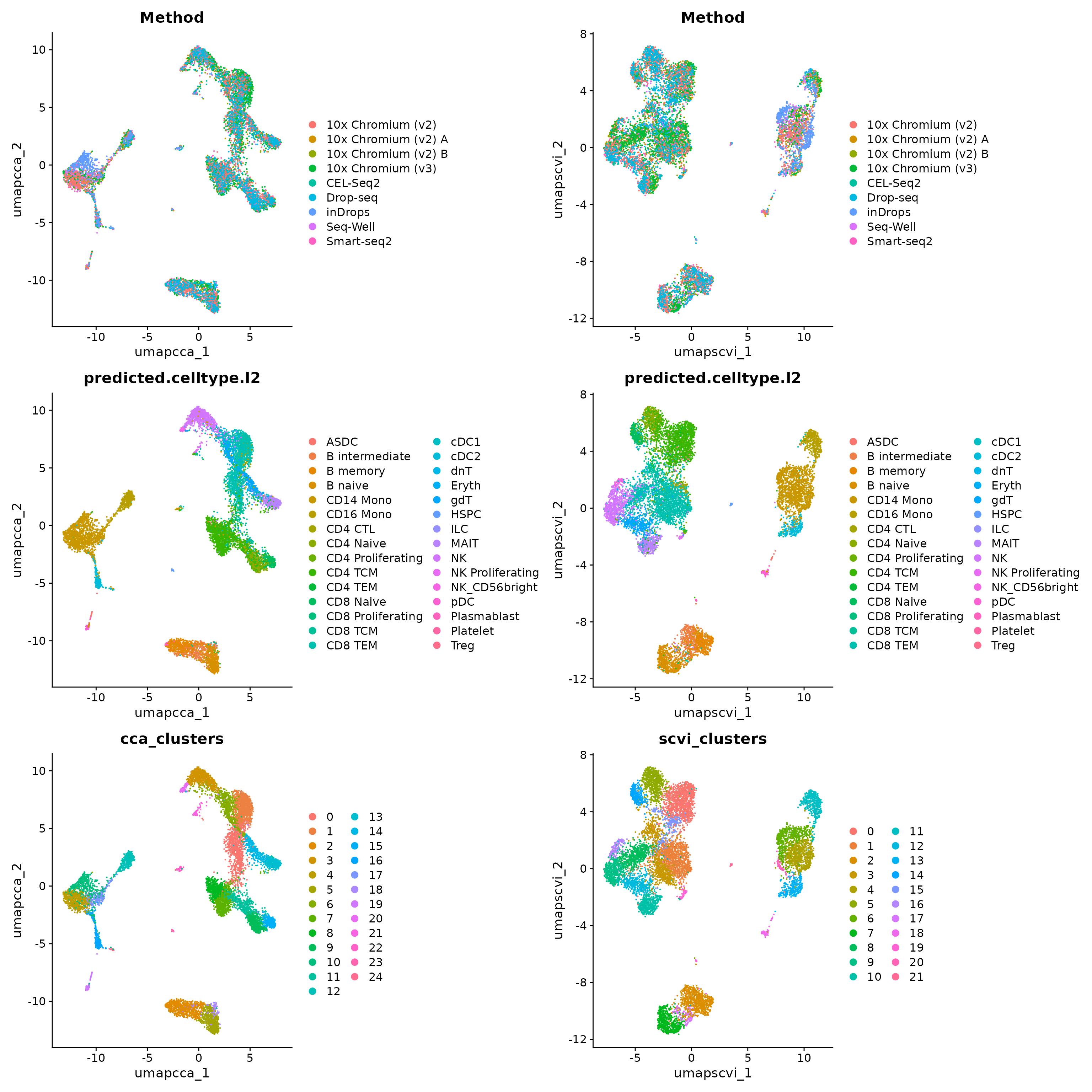
We hope that by simplifying the process of performing integrative analysis, users can more carefully evaluate the biological information retained in the integrated dataset. For example, users can compare the expression of biological markers based on different clustering solutions, or visualize one method’s clustering solution on different UMAP visualizations.
p1 <- VlnPlot(obj, features = "rna_CD8A", group.by = "unintegrated_clusters") + NoLegend() +
    ggtitle("CD8A - Unintegrated Clusters")
p2 <- VlnPlot(obj, "rna_CD8A", group.by = "cca_clusters") + NoLegend() + ggtitle("CD8A - CCA Clusters")
p3 <- VlnPlot(obj, "rna_CD8A", group.by = "scvi_clusters") + NoLegend() + ggtitle("CD8A - scVI Clusters")
p1 | p2 | p3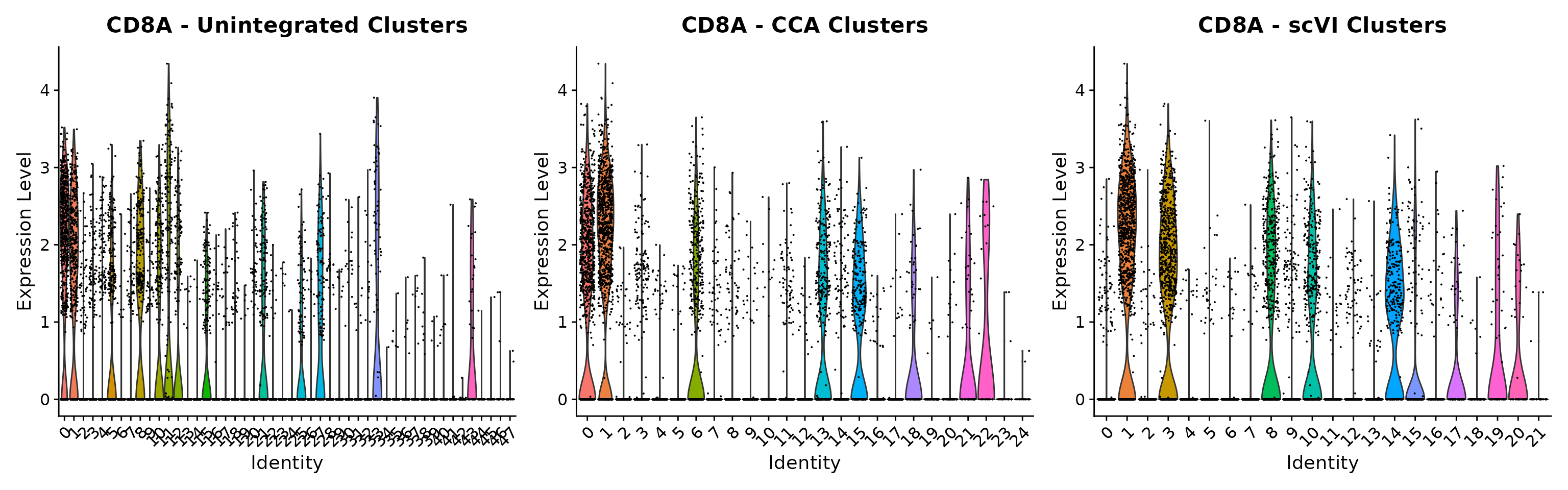
obj <- RunUMAP(obj, reduction = "integrated.rpca", dims = 1:30, reduction.name = "umap.rpca")
p4 <- DimPlot(obj, reduction = "umap.unintegrated", group.by = c("cca_clusters"))
p5 <- DimPlot(obj, reduction = "umap.rpca", group.by = c("cca_clusters"))
p6 <- DimPlot(obj, reduction = "umap.scvi", group.by = c("cca_clusters"))
p4 | p5 | p6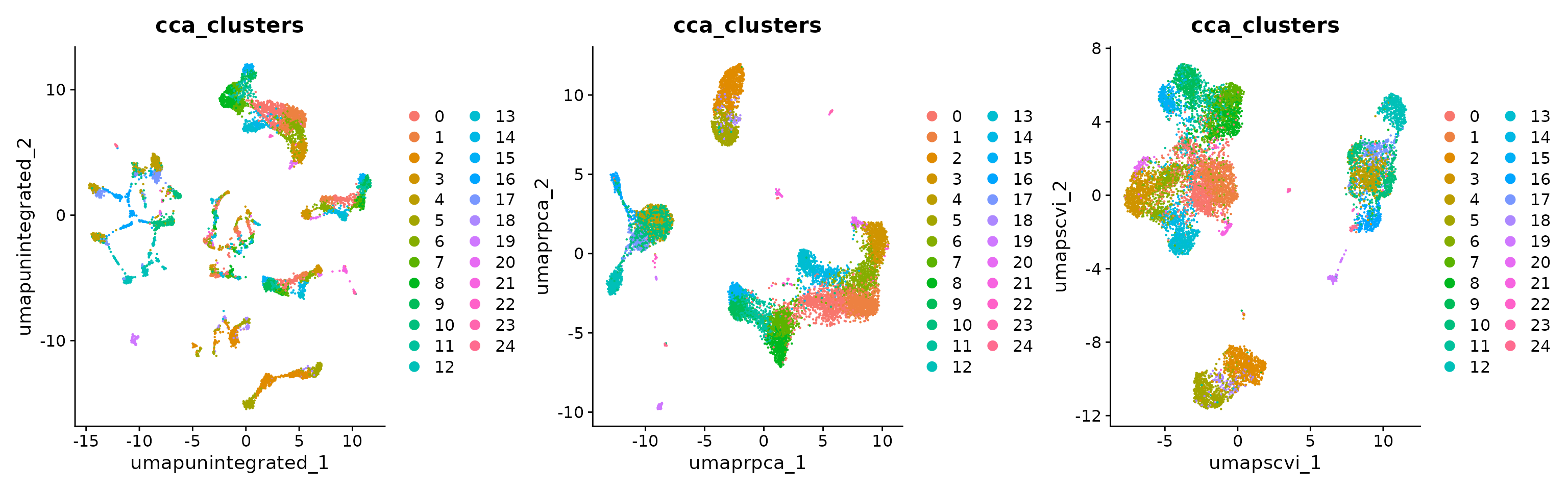
Once integrative analysis is complete, you can rejoin the layers -
which collapses the individual datasets together and recreates the
original counts and data layers. You will need
to do this before performing any differential expression analysis.
However, you can always resplit the layers in case you would like to
reperform integrative analysis.
obj <- JoinLayers(obj)
obj
## An object of class Seurat
## 35789 features across 10434 samples within 5 assays
## Active assay: RNA (33694 features, 2000 variable features)
## 3 layers present: data, counts, scale.data
## 4 other assays present: prediction.score.celltype.l1, prediction.score.celltype.l2, prediction.score.celltype.l3, mnn.reconstructed
## 12 dimensional reductions calculated: integrated_dr, ref.umap, pca, umap.unintegrated, integrated.cca, integrated.rpca, harmony, integrated.mnn, integrated.scvi, umap.cca, umap.scvi, umap.rpcaLastly, users can also perform integration using
sctransform-normalized data (see our SCTransform
vignette for more information), by first running SCTransform
normalization, and then setting the normalization.method
argument in IntegrateLayers.
obj <- SCTransform(obj)
obj <- RunPCA(obj, npcs = 30, verbose = F)
obj <- IntegrateLayers(object = obj, method = RPCAIntegration, normalization.method = "SCT",
    verbose = F)
obj <- FindNeighbors(obj, dims = 1:30, reduction = "integrated.dr")
obj <- FindClusters(obj, resolution = 2)
## Modularity Optimizer version 1.3.0 by Ludo Waltman and Nees Jan van Eck
##
## Number of nodes: 10434
## Number of edges: 445061
##
## Running Louvain algorithm...
## Maximum modularity in 10 random starts: 0.8359
## Number of communities: 27
## Elapsed time: 1 seconds
obj <- RunUMAP(obj, dims = 1:30, reduction = "integrated.dr")Session Info
## R version 4.5.2 (2025-10-31)
## Platform: x86_64-pc-linux-gnu
## Running under: Ubuntu 24.04.4 LTS
##
## Matrix products: default
## BLAS:   /usr/lib/x86_64-linux-gnu/openblas-pthread/libblas.so.3
## LAPACK: /usr/lib/x86_64-linux-gnu/openblas-pthread/libopenblasp-r0.3.26.so;  LAPACK version 3.12.0
##
## locale:
##  [1] LC_CTYPE=en_US.UTF-8       LC_NUMERIC=C
##  [3] LC_TIME=en_US.UTF-8        LC_COLLATE=en_US.UTF-8
##  [5] LC_MONETARY=en_US.UTF-8    LC_MESSAGES=en_US.UTF-8
##  [7] LC_PAPER=en_US.UTF-8       LC_NAME=C
##  [9] LC_ADDRESS=C               LC_TELEPHONE=C
## [11] LC_MEASUREMENT=en_US.UTF-8 LC_IDENTIFICATION=C
##
## time zone: Etc/UTC
## tzcode source: system (glibc)
##
## attached base packages:
## [1] stats     graphics  grDevices utils     datasets  methods   base
##
## other attached packages:
##  [1] future_1.70.0            patchwork_1.3.2          ggplot2_4.0.3
##  [4] Azimuth_0.5.1            shinyBS_0.65.0           SeuratWrappers_0.4.0
##  [7] pbmcsca.SeuratData_3.0.0 pbmcref.SeuratData_1.0.0 SeuratData_0.2.2.9002
## [10] Seurat_5.5.0             SeuratObject_5.4.0       sp_2.2-1
##
## loaded via a namespace (and not attached):
##   [1] fs_2.1.0                          ProtGenerics_1.42.0
##   [3] matrixStats_1.5.0                 spatstat.sparse_3.1-0
##   [5] bitops_1.0-9                      DirichletMultinomial_1.52.0
##   [7] TFBSTools_1.48.0                  httr_1.4.8
##   [9] RColorBrewer_1.1-3                tools_4.5.2
##  [11] sctransform_0.4.3                 ResidualMatrix_1.20.0
##  [13] R6_2.6.1                          DT_0.34.0
##  [15] lazyeval_0.2.3                    uwot_0.2.4
##  [17] rhdf5filters_1.22.0               withr_3.0.2
##  [19] gridExtra_2.3                     progressr_0.19.0
##  [21] cli_3.6.6                         Biobase_2.70.0
##  [23] textshaping_1.0.5                 formatR_1.14
##  [25] spatstat.explore_3.8-0            fastDummies_1.7.6
##  [27] EnsDb.Hsapiens.v86_2.99.0         shinyjs_2.1.1
##  [29] labeling_0.4.3                    sass_0.4.10
##  [31] S7_0.2.1                          spatstat.data_3.1-9
##  [33] ggridges_0.5.7                    pbapply_1.7-4
##  [35] pkgdown_2.2.0                     Rsamtools_2.26.0
##  [37] systemfonts_1.3.2                 R.utils_2.13.0
##  [39] harmony_2.0.2                     parallelly_1.47.0
##  [41] BSgenome_1.78.0                   RSQLite_2.4.6
##  [43] generics_0.1.4                    BiocIO_1.20.0
##  [45] gtools_3.9.5                      ica_1.0-3
##  [47] spatstat.random_3.4-5             googlesheets4_1.1.2
##  [49] dplyr_1.2.0                       Matrix_1.7-5
##  [51] ggbeeswarm_0.7.3                  S4Vectors_0.48.1
##  [53] abind_1.4-8                       R.methodsS3_1.8.2
##  [55] lifecycle_1.0.5                   yaml_2.3.12
##  [57] SummarizedExperiment_1.40.0       glmGamPoi_1.22.0
##  [59] rhdf5_2.54.1                      SparseArray_1.10.10
##  [61] Rtsne_0.17                        grid_4.5.2
##  [63] blob_1.3.0                        promises_1.5.0
##  [65] shinydashboard_0.7.3              pwalign_1.6.0
##  [67] crayon_1.5.3                      miniUI_0.1.2
##  [69] lattice_0.22-7                    beachmat_2.26.0
##  [71] cowplot_1.2.0                     GenomicFeatures_1.62.0
##  [73] cigarillo_1.0.0                   KEGGREST_1.50.0
##  [75] pillar_1.11.1                     knitr_1.51
##  [77] GenomicRanges_1.62.1              rjson_0.2.23
##  [79] future.apply_1.20.2               codetools_0.2-20
##  [81] fastmatch_1.1-8                   glue_1.8.0
##  [83] spatstat.univar_3.1-7             data.table_1.18.2.1
##  [85] remotes_2.5.0                     vctrs_0.7.1
##  [87] png_0.1-9                         spam_2.11-3
##  [89] cellranger_1.1.0                  gtable_0.3.6
##  [91] cachem_1.1.0                      xfun_0.56
##  [93] Signac_1.17.1                     S4Arrays_1.10.1
##  [95] mime_0.13                         Seqinfo_1.0.0
##  [97] survival_3.8-3                    gargle_1.6.1
##  [99] SingleCellExperiment_1.32.0       RcppRoll_0.3.2
## [101] fitdistrplus_1.2-6                ROCR_1.0-12
## [103] nlme_3.1-168                      bit64_4.6.0-1
## [105] RcppAnnoy_0.0.23                  GenomeInfoDb_1.46.2
## [107] bslib_0.10.0                      irlba_2.3.7
## [109] vipor_0.4.7                       KernSmooth_2.23-26
## [111] otel_0.2.0                        SeuratDisk_0.0.0.9021
## [113] seqLogo_1.76.0                    BiocGenerics_0.56.0
## [115] DBI_1.3.0                         ggrastr_1.0.2
## [117] tidyselect_1.2.1                  bit_4.6.0
## [119] compiler_4.5.2                    curl_7.0.0
## [121] BiocNeighbors_2.4.0               hdf5r_1.3.12
## [123] desc_1.4.3                        DelayedArray_0.36.1
## [125] plotly_4.12.0                     rtracklayer_1.70.1
## [127] scales_1.4.0                      caTools_1.18.3
## [129] lmtest_0.9-40                     rappdirs_0.3.4
## [131] stringr_1.6.0                     digest_0.6.39
## [133] goftest_1.2-3                     presto_1.0.0
## [135] spatstat.utils_3.2-2              rmarkdown_2.30
## [137] RhpcBLASctl_0.23-42               XVector_0.50.0
## [139] htmltools_0.5.9                   pkgconfig_2.0.3
## [141] sparseMatrixStats_1.22.0          MatrixGenerics_1.22.0
## [143] fastmap_1.2.0                     ensembldb_2.34.0
## [145] rlang_1.2.0                       htmlwidgets_1.6.4
## [147] UCSC.utils_1.6.1                  DelayedMatrixStats_1.32.0
## [149] shiny_1.13.0                      farver_2.1.2
## [151] jquerylib_0.1.4                   zoo_1.8-15
## [153] jsonlite_2.0.0                    BiocParallel_1.44.0
## [155] R.oo_1.27.1                       BiocSingular_1.26.1
## [157] RCurl_1.98-1.18                   magrittr_2.0.5
## [159] scuttle_1.20.0                    dotCall64_1.2
## [161] Rhdf5lib_1.32.0                   Rcpp_1.1.1-1.1
## [163] reticulate_1.46.0                 stringi_1.8.7
## [165] MASS_7.3-65                       plyr_1.8.9
## [167] parallel_4.5.2                    listenv_0.10.1
## [169] ggrepel_0.9.8                     deldir_2.0-4
## [171] Biostrings_2.78.0                 splines_4.5.2
## [173] tensor_1.5.1                      BSgenome.Hsapiens.UCSC.hg38_1.4.5
## [175] igraph_2.3.0                      spatstat.geom_3.7-3
## [177] RcppHNSW_0.6.0                    ScaledMatrix_1.18.0
## [179] reshape2_1.4.5                    stats4_4.5.2
## [181] TFMPvalue_1.0.0                   XML_3.99-0.23
## [183] evaluate_1.0.5                    BiocManager_1.30.27
## [185] batchelor_1.26.0                  JASPAR2020_0.99.10
## [187] httpuv_1.6.16                     RANN_2.6.2
## [189] tidyr_1.3.2                       purrr_1.2.1
## [191] polyclip_1.10-7                   scattermore_1.2
## [193] rsvd_1.0.5                        xtable_1.8-8
## [195] restfulr_0.0.16                   AnnotationFilter_1.34.0
## [197] RSpectra_0.16-2                   later_1.4.8
## [199] googledrive_2.1.2                 viridisLite_0.4.3
## [201] ragg_1.5.1                        tibble_3.3.1
## [203] beeswarm_0.4.0                    memoise_2.0.1
## [205] AnnotationDbi_1.72.0              GenomicAlignments_1.46.0
## [207] IRanges_2.44.0                    cluster_2.1.8.2
## [209] globals_0.19.1