Using BPCells with Seurat Objects

BPCells is an R package that allows for computationally efficient single-cell analysis. It utilizes bit-packing compression to store counts matrices on disk and C++ code to cache operations.

We leverage the high performance capabilities of BPCells to work with Seurat objects in memory while accessing the counts on disk. In this vignette, we show how to use BPCells to load data, work with a Seurat objects in a more memory-efficient way, and write out Seurat objects with BPCells matrices.

We will show the methods for interacting with both a single dataset in one file or multiple datasets across multiple files using BPCells. BPCells allows us to easily analyze these large datasets in memory, and we encourage users to check out some of our other vignettes here and here to see further applications.

library(BPCells)
library(Seurat)
library(SeuratObject)
library(SeuratDisk)
library(Azimuth)

We use BPCells functionality to both load in our data and write the counts layers to bitpacked compressed binary files on disk to improve computation speeds. BPCells has multiple functions for reading in files.

Load Data

Load Data from one h5 file

In this section, we will load a dataset of mouse brain cells freely available from 10x Genomics. This includes 1.3 Million single cells that were sequenced on the Illumina NovaSeq 6000. The raw data can be found here.

To read in the file, we will use open_matrix_10x_hdf5, a BPCells function written to read in feature matrices from 10x. We then write a matrix directory, load the matrix, and create a Seurat object.

brain.data <- open_matrix_10x_hdf5(
  path = "/brahms/hartmana/vignette_data/1M_neurons_filtered_gene_bc_matrices_h5.h5"
)
# Write the matrix to a directory
 write_matrix_dir(
   mat = brain.data,
   dir = '/brahms/hartmana/vignette_data/bpcells/brain_counts')
# Now that we have the matrix on disk, we can load it
brain.mat <- open_matrix_dir(dir = "/brahms/hartmana/vignette_data/bpcells/brain_counts")
brain.mat <- Azimuth:::ConvertEnsembleToSymbol(mat = brain.mat, species = "mouse")

# Create Seurat Object
brain <- CreateSeuratObject(counts = brain.mat)

What if I already have a Seurat Object?

You can use BPCells to convert the matrices in your already created Seurat objects to on-disk matrices. Note, that this is only possible for V5 assays. As an example, if you’d like to convert the counts matrix of your RNA assay to a BPCells matrix, you can use the following:

# obj <- readRDS("/path/to/reference.rds")

# # Write the counts layer to a directory
 write_matrix_dir(mat = obj[["RNA"]]$counts, dir = '/brahms/hartmana/vignette_data/bpcells/brain_counts')
 counts.mat <- open_matrix_dir(dir = "/brahms/hartmana/vignette_data/bpcells/brain_counts")

# obj[["RNA"]]$counts <- counts.mat

Example Analsyis

Once this conversion is done, you can perform typical Seurat functions on the object. For example, we can normalize data and visualize features by automatically accessing the on-disk counts.

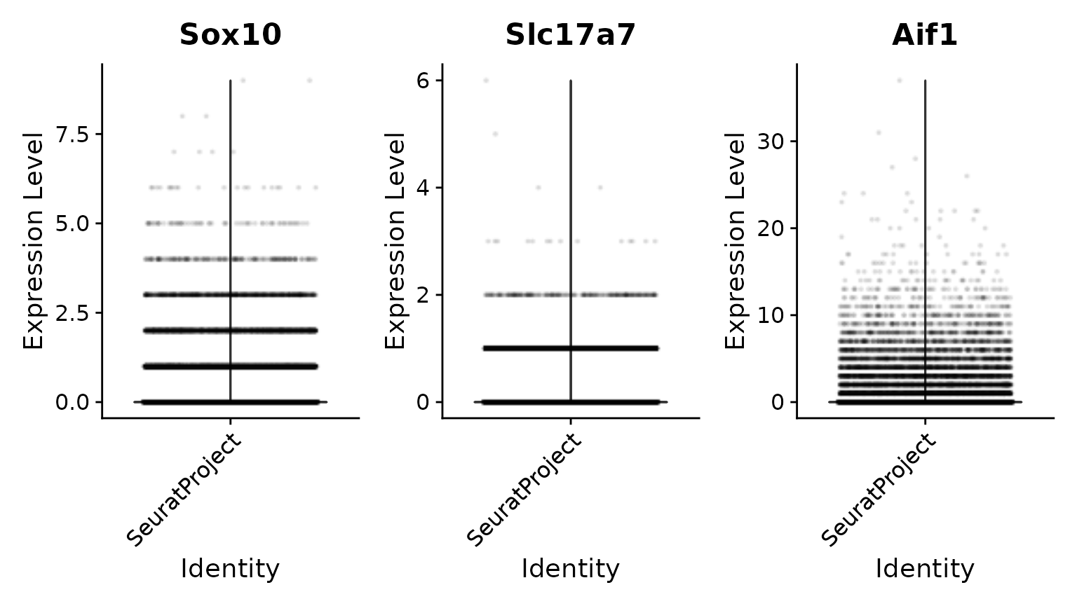
VlnPlot(brain, features = c("Sox10", "Slc17a7", "Aif1"), ncol = 3, layer = "counts", alpha = 0.1)

# We then normalize and visualize again
brain <- NormalizeData(brain, normalization.method = "LogNormalize")
VlnPlot(brain, features = c("Sox10", "Slc17a7", "Aif1"), ncol = 3, layer = "data", alpha = 0.1)

Saving Seurat objects with on-disk layers

If you save your object and load it in in the future, Seurat will access the on-disk matrices by their path, which is stored in the assay level data. saveRDS() can still be used to save your Seurat objects with on-disk matrices as shown below. Note, if you move the object across computers or to a place that no longer has access to the paths where the on-disk matrices are stored, you will have to move the folders that contain the on-disk matrices as well. We are actively working on functionality to make this process easier for users.

saveRDS(
   object = brain,
   file = "obj.Rds"
)

If needed, a layer with an on-disk matrix can be converted to an in-memory matrix using the as() function. For the purposes of this demo, we’ll subset the object so that it takes up less space in memory.

brain <- subset(brain, downsample = 1000)
brain[["RNA"]]$counts <- as(object = brain[["RNA"]]$counts, Class = "dgCMatrix")

Load data from multiple h5ad files

You can also download data from multiple matrices. In this section, we create a Seurat object using multiple peripheral blood mononuclear cell (PBMC) samples that are freely available for download from CZI here. We download data from Ahern et al. (2022) Nature, Jin et al. (2021) Science, and Yoshida et al. (2022) Nature. We use the BPCells function to read h5ad files.

file.dir <- "/brahms/hartmana/vignette_data/h5ad_files/"
files.set <- c("ahern_pbmc.h5ad", "jin_pbmc.h5ad", "yoshida_pbmc.h5ad")

# Loop through h5ad files and output BPCells matrices on-disk
data.list <- c()
metadata.list <- c()

for (i in 1:length(files.set)) {
  path <- paste0(file.dir, files.set[i])
  data <- open_matrix_anndata_hdf5(path)
   write_matrix_dir(
     mat = data,
     dir = paste0(gsub(".h5ad", "", path), "_BP")
   )
  # Load in BP matrices
  mat <- open_matrix_dir(dir = paste0(gsub(".h5ad", "", path), "_BP"))
  mat <- Azimuth:::ConvertEnsembleToSymbol(mat = mat, species = "human")
  # Get metadata
  metadata.list[[i]] <- LoadH5ADobs(path = path)
  data.list[[i]] <- mat
}
# Name layers
names(data.list) <- c("ahern", "jin", "yoshida")

# Add Metadata
for (i in 1:length(metadata.list)) {
  metadata.list[[i]]$publication <- names(data.list)[i]
}
metadata.list <- lapply(metadata.list, function(x) {
  x <- x[, c("publication", "sex", "cell_type", "donor_id", "disease")]
  return(x)
})
metadata <- Reduce(rbind, metadata.list)

When we create the Seurat object with the list of matrices from each publication, we can then see that multiple counts layers exist that represent each dataset. This object contains over a million cells, yet only takes up minimal space in memory!

merged.object <- CreateSeuratObject(counts = data.list, meta.data = metadata)
merged.object

## An object of class Seurat 
## 26143 features across 1498064 samples within 1 assay 
## Active assay: RNA (26143 features, 0 variable features)
##  3 layers present: counts.ahern, counts.jin, counts.yoshida

saveRDS(
  object = merged.object,
  file = "obj.Rds"
)

Parse Biosciences

Here, we show how to load a 1 million cell data set from Parse Biosciences and create a Seurat Object. The data is available for download here

parse.data <- open_matrix_anndata_hdf5(
  "/brahms/hartmana/vignette_data/h5ad_files/ParseBio_PBMC.h5ad"
)

write_matrix_dir(mat = parse.data, dir = "/brahms/hartmana/vignette_data/bpcells/parse_1m_pbmc")

parse.mat <- open_matrix_dir(dir = "/brahms/hartmana/vignette_data/bpcells/parse_1m_pbmc")
metadata <- readRDS("/brahms/hartmana/vignette_data/ParseBio_PBMC_meta.rds")
metadata$disease <- sapply(strsplit(x = metadata$sample, split = "_"), "[", 1)
parse.object <- CreateSeuratObject(counts = parse.mat, meta.data = metadata)

saveRDS(
  object = parse.object,
  file = "obj.Rds"
)

Session Info

sessionInfo()