Fast integration using reciprocal PCA (RPCA)
Compiled: October 31, 2023
Source:vignettes/integration_rpca.Rmd
integration_rpca.RmdIn this vignette, we present a slightly modified workflow for the integration of scRNA-seq datasets. Instead of utilizing canonical correlation analysis (‘CCA’) to identify anchors, we instead utilize reciprocal PCA (‘RPCA’). When determining anchors between any two datasets using RPCA, we project each dataset into the others PCA space and constrain the anchors by the same mutual neighborhood requirement. The commands for both workflows are largely identical, but the two methods may be applied in different context.
By identifying shared sources of variation between datasets, CCA is well-suited for identifying anchors when cell types are conserved, but there are very substantial differences in gene expression across experiments. CCA-based integration therefore enables integrative analysis when experimental conditions or disease states introduce very strong expression shifts, or when integrating datasets across modalities and species. However, CCA-based integration may also lead to overcorrection, especially when a large proportion of cells are non-overlapping across datasets.
RPCA-based integration runs significantly faster, and also represents a more conservative approach where cells in different biological states are less likely to ‘align’ after integration. We therefore recommend RPCA during integrative analysis where:
- A substantial fraction of cells in one dataset have no matching type in the other
- Datasets originate from the same platform (i.e. multiple lanes of 10x genomics)
- There are a large number of datasets or cells to integrate (see here for more tips on integrating large datasets)
Below, we demonstrate the use of reciprocal PCA to align the same stimulated and resting datasets first analyzed in our introduction to scRNA-seq integration vignette. While the list of commands is nearly identical, this workflow requires users to run principal components analysis (PCA) individually on each dataset prior to integration. Users should also set the ‘reduction’ argument to ‘rpca’, when running FindIntegrationAnchors().
library(Seurat)
library(SeuratData)
# install dataset
InstallData("ifnb")
# load dataset
ifnb <- LoadData("ifnb")

# split the dataset into a list of two seurat objects (stim and CTRL)
ifnb.list <- SplitObject(ifnb, split.by = "stim")

# normalize and identify variable features for each dataset independently
ifnb.list <- lapply(X = ifnb.list, FUN = function(x) {
    x <- NormalizeData(x)
    x <- FindVariableFeatures(x, selection.method = "vst", nfeatures = 2000)
})

# select features that are repeatedly variable across datasets for integration run PCA on each
# dataset using these features
features <- SelectIntegrationFeatures(object.list = ifnb.list)
ifnb.list <- lapply(X = ifnb.list, FUN = function(x) {
    x <- ScaleData(x, features = features, verbose = FALSE)
    x <- RunPCA(x, features = features, verbose = FALSE)
})
Perform integration
We then identify anchors using the FindIntegrationAnchors() function, which takes a list of Seurat objects as input, and use these anchors to integrate the two datasets together with IntegrateData().
immune.anchors <- FindIntegrationAnchors(object.list = ifnb.list, anchor.features = features, reduction = "rpca")
# this command creates an 'integrated' data assay
immune.combined <- IntegrateData(anchorset = immune.anchors)
Now we can run a single integrated analysis on all cells!
# specify that we will perform downstream analysis on the corrected data note that the
# original unmodified data still resides in the 'RNA' assay
DefaultAssay(immune.combined) <- "integrated"

# Run the standard workflow for visualization and clustering
immune.combined <- ScaleData(immune.combined, verbose = FALSE)
immune.combined <- RunPCA(immune.combined, npcs = 30, verbose = FALSE)
immune.combined <- RunUMAP(immune.combined, reduction = "pca", dims = 1:30)
immune.combined <- FindNeighbors(immune.combined, reduction = "pca", dims = 1:30)
immune.combined <- FindClusters(immune.combined, resolution = 0.5)
# Visualization
p1 <- DimPlot(immune.combined, reduction = "umap", group.by = "stim")
p2 <- DimPlot(immune.combined, reduction = "umap", group.by = "seurat_annotations", label = TRUE,
    repel = TRUE)
p1 + p2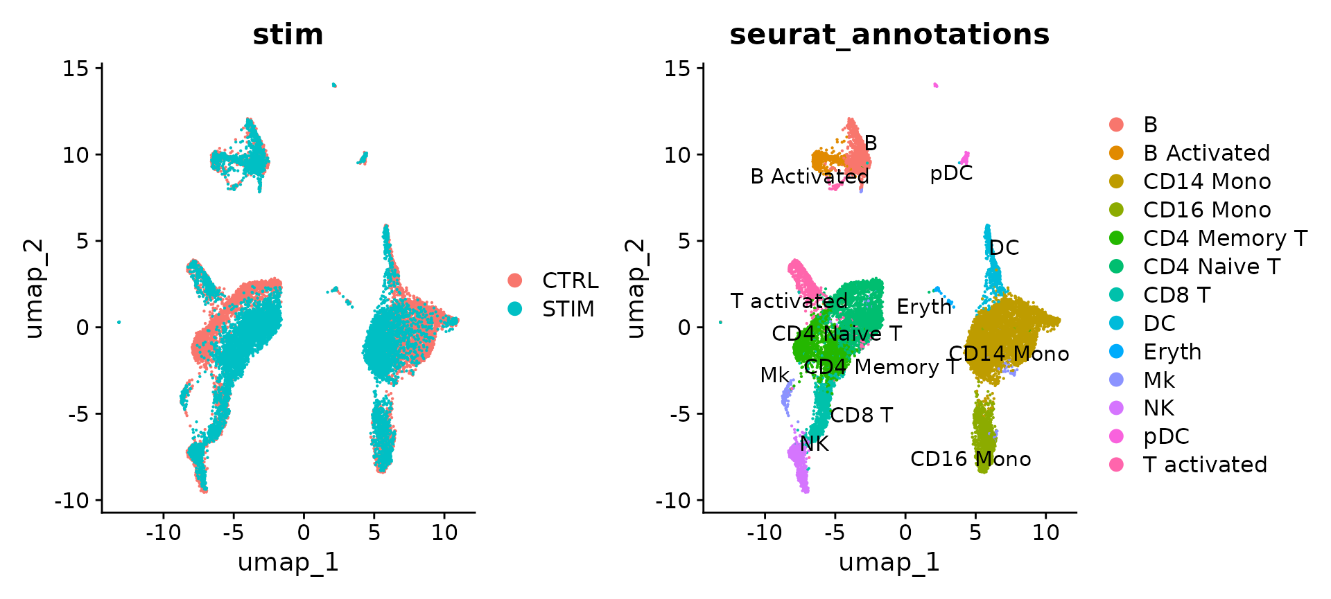
Modifying the strength of integration
The results show that rpca-based integration is more conservative, and in this case, do not perfectly align a subset of cells (which are naive and memory T cells) across experiments. You can increase the strength of alignment by increasing the k.anchor parameter, which is set to 5 by default. Increasing this parameter to 20 will assist in aligning these populations.
immune.anchors <- FindIntegrationAnchors(object.list = ifnb.list, anchor.features = features, reduction = "rpca",
    k.anchor = 20)
immune.combined <- IntegrateData(anchorset = immune.anchors)

immune.combined <- ScaleData(immune.combined, verbose = FALSE)
immune.combined <- RunPCA(immune.combined, npcs = 30, verbose = FALSE)
immune.combined <- RunUMAP(immune.combined, reduction = "pca", dims = 1:30)
immune.combined <- FindNeighbors(immune.combined, reduction = "pca", dims = 1:30)
immune.combined <- FindClusters(immune.combined, resolution = 0.5)
## Modularity Optimizer version 1.3.0 by Ludo Waltman and Nees Jan van Eck
##
## Number of nodes: 13999
## Number of edges: 594845
##
## Running Louvain algorithm...
## Maximum modularity in 10 random starts: 0.9098
## Number of communities: 15
## Elapsed time: 2 seconds
# Visualization
p1 <- DimPlot(immune.combined, reduction = "umap", group.by = "stim")
p2 <- DimPlot(immune.combined, reduction = "umap", label = TRUE, repel = TRUE)
p1 + p2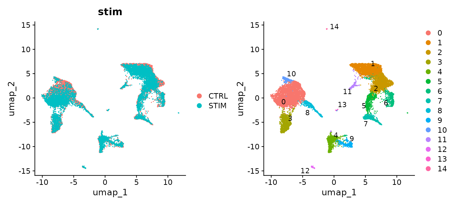
library(ggplot2)
plot <- DimPlot(immune.combined, group.by = "stim") + xlab("UMAP 1") + ylab("UMAP 2") + theme(axis.title = element_text(size = 18),
    legend.text = element_text(size = 18)) + guides(colour = guide_legend(override.aes = list(size = 10)))
ggsave(filename = "../output/images/rpca_integration.jpg", height = 7, width = 12, plot = plot,
    quality = 50)
Now that the datasets have been integrated, you can follow the previous steps in the introduction to scRNA-seq integration vignette to identify cell types and cell type-specific responses.
Performing integration on datasets normalized with SCTransform
As an additional example, we repeat the analyses performed above, but normalize the datasets using SCTransform. We may choose to set the method parameter to glmGamPoi (install here) in order to enable faster estimation of regression parameters in SCTransform().
ifnb <- LoadData("ifnb")
ifnb.list <- SplitObject(ifnb, split.by = "stim")
ifnb.list <- lapply(X = ifnb.list, FUN = SCTransform, method = "glmGamPoi")
features <- SelectIntegrationFeatures(object.list = ifnb.list, nfeatures = 3000)
ifnb.list <- PrepSCTIntegration(object.list = ifnb.list, anchor.features = features)
ifnb.list <- lapply(X = ifnb.list, FUN = RunPCA, features = features)
immune.anchors <- FindIntegrationAnchors(object.list = ifnb.list, normalization.method = "SCT",
    anchor.features = features, dims = 1:30, reduction = "rpca", k.anchor = 20)
immune.combined.sct <- IntegrateData(anchorset = immune.anchors, normalization.method = "SCT", dims = 1:30)
## [1] 1
## [1] 2
immune.combined.sct <- RunPCA(immune.combined.sct, verbose = FALSE)
immune.combined.sct <- RunUMAP(immune.combined.sct, reduction = "pca", dims = 1:30)
# Visualization
p1 <- DimPlot(immune.combined.sct, reduction = "umap", group.by = "stim")
p2 <- DimPlot(immune.combined.sct, reduction = "umap", group.by = "seurat_annotations", label = TRUE,
    repel = TRUE)
p1 + p2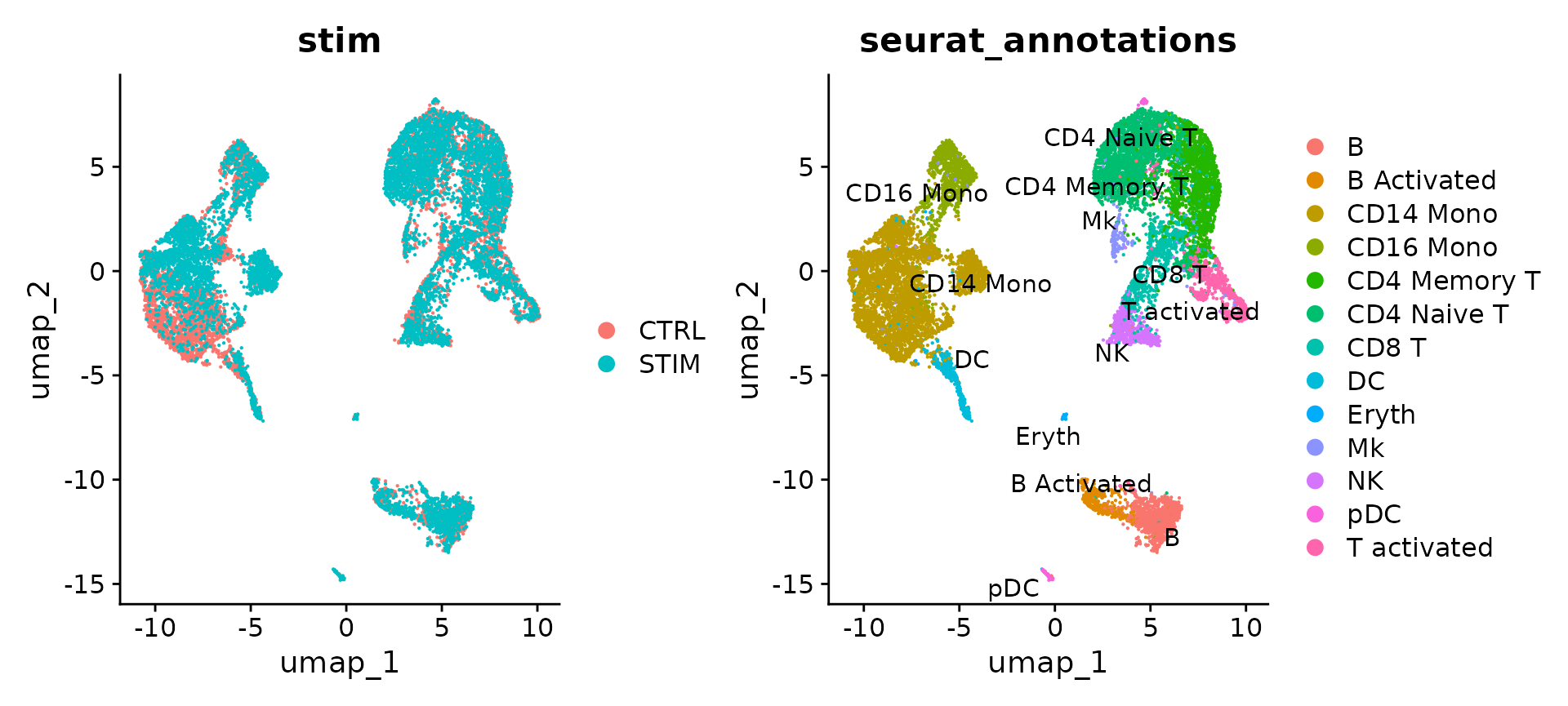
Session Info
## R version 4.2.2 Patched (2022-11-10 r83330)
## Platform: x86_64-pc-linux-gnu (64-bit)
## Running under: Ubuntu 20.04.6 LTS
##
## Matrix products: default
## BLAS:   /usr/lib/x86_64-linux-gnu/blas/libblas.so.3.9.0
## LAPACK: /usr/lib/x86_64-linux-gnu/lapack/liblapack.so.3.9.0
##
## locale:
##  [1] LC_CTYPE=en_US.UTF-8       LC_NUMERIC=C
##  [3] LC_TIME=en_US.UTF-8        LC_COLLATE=en_US.UTF-8
##  [5] LC_MONETARY=en_US.UTF-8    LC_MESSAGES=en_US.UTF-8
##  [7] LC_PAPER=en_US.UTF-8       LC_NAME=C
##  [9] LC_ADDRESS=C               LC_TELEPHONE=C
## [11] LC_MEASUREMENT=en_US.UTF-8 LC_IDENTIFICATION=C
##
## attached base packages:
## [1] stats     graphics  grDevices utils     datasets  methods   base
##
## other attached packages:
##  [1] ggplot2_3.4.4                 thp1.eccite.SeuratData_3.1.5
##  [3] stxBrain.SeuratData_0.1.1     ssHippo.SeuratData_3.1.4
##  [5] pbmcsca.SeuratData_3.0.0      pbmcref.SeuratData_1.0.0
##  [7] pbmcMultiome.SeuratData_0.1.4 pbmc3k.SeuratData_3.1.4
##  [9] panc8.SeuratData_3.0.2        ifnb.SeuratData_3.0.0
## [11] hcabm40k.SeuratData_3.0.0     cbmc.SeuratData_3.1.4
## [13] bmcite.SeuratData_0.3.0       SeuratData_0.2.2.9001
## [15] Seurat_5.0.0                  SeuratObject_5.0.0
## [17] sp_2.1-1
##
## loaded via a namespace (and not attached):
##   [1] spam_2.10-0                 systemfonts_1.0.4
##   [3] plyr_1.8.9                  igraph_1.5.1
##   [5] lazyeval_0.2.2              splines_4.2.2
##   [7] RcppHNSW_0.5.0              listenv_0.9.0
##   [9] scattermore_1.2             GenomeInfoDb_1.34.9
##  [11] digest_0.6.33               htmltools_0.5.6.1
##  [13] fansi_1.0.5                 magrittr_2.0.3
##  [15] memoise_2.0.1               tensor_1.5
##  [17] cluster_2.1.4               ROCR_1.0-11
##  [19] globals_0.16.2              matrixStats_1.0.0
##  [21] pkgdown_2.0.7               spatstat.sparse_3.0-3
##  [23] colorspace_2.1-0            rappdirs_0.3.3
##  [25] ggrepel_0.9.4               textshaping_0.3.6
##  [27] xfun_0.40                   dplyr_1.1.3
##  [29] RCurl_1.98-1.12             crayon_1.5.2
##  [31] jsonlite_1.8.7              progressr_0.14.0
##  [33] spatstat.data_3.0-3         survival_3.5-7
##  [35] zoo_1.8-12                  glue_1.6.2
##  [37] polyclip_1.10-6             gtable_0.3.4
##  [39] zlibbioc_1.44.0             XVector_0.38.0
##  [41] leiden_0.4.3                DelayedArray_0.24.0
##  [43] future.apply_1.11.0         BiocGenerics_0.44.0
##  [45] abind_1.4-5                 scales_1.2.1
##  [47] spatstat.random_3.2-1       miniUI_0.1.1.1
##  [49] Rcpp_1.0.11                 viridisLite_0.4.2
##  [51] xtable_1.8-4                reticulate_1.34.0
##  [53] dotCall64_1.1-0             stats4_4.2.2
##  [55] htmlwidgets_1.6.2           httr_1.4.7
##  [57] RColorBrewer_1.1-3          ellipsis_0.3.2
##  [59] ica_1.0-3                   farver_2.1.1
##  [61] pkgconfig_2.0.3             sass_0.4.7
##  [63] uwot_0.1.16                 deldir_1.0-9
##  [65] utf8_1.2.4                  labeling_0.4.3
##  [67] tidyselect_1.2.0            rlang_1.1.1
##  [69] reshape2_1.4.4              later_1.3.1
##  [71] munsell_0.5.0               tools_4.2.2
##  [73] cachem_1.0.8                cli_3.6.1
##  [75] generics_0.1.3              ggridges_0.5.4
##  [77] evaluate_0.22               stringr_1.5.0
##  [79] fastmap_1.1.1               yaml_2.3.7
##  [81] ragg_1.2.5                  goftest_1.2-3
##  [83] knitr_1.45                  fs_1.6.3
##  [85] fitdistrplus_1.1-11         purrr_1.0.2
##  [87] RANN_2.6.1                  sparseMatrixStats_1.10.0
##  [89] pbapply_1.7-2               future_1.33.0
##  [91] nlme_3.1-162                mime_0.12
##  [93] formatR_1.14                compiler_4.2.2
##  [95] plotly_4.10.3               png_0.1-8
##  [97] spatstat.utils_3.0-4        tibble_3.2.1
##  [99] glmGamPoi_1.10.2            bslib_0.5.1
## [101] stringi_1.7.12              highr_0.10
## [103] desc_1.4.2                  RSpectra_0.16-1
## [105] lattice_0.21-9              Matrix_1.6-1.1
## [107] vctrs_0.6.4                 pillar_1.9.0
## [109] lifecycle_1.0.3             spatstat.geom_3.2-7
## [111] lmtest_0.9-40               jquerylib_0.1.4
## [113] RcppAnnoy_0.0.21            bitops_1.0-7
## [115] data.table_1.14.8           cowplot_1.1.1
## [117] irlba_2.3.5.1               GenomicRanges_1.50.2
## [119] httpuv_1.6.12               patchwork_1.1.3
## [121] R6_2.5.1                    promises_1.2.1
## [123] KernSmooth_2.23-22          gridExtra_2.3
## [125] IRanges_2.32.0              parallelly_1.36.0
## [127] codetools_0.2-19            fastDummies_1.7.3
## [129] MASS_7.3-58.2               SummarizedExperiment_1.28.0
## [131] rprojroot_2.0.3             withr_2.5.2
## [133] sctransform_0.4.1           GenomeInfoDbData_1.2.9
## [135] S4Vectors_0.36.2            parallel_4.2.2
## [137] grid_4.2.2                  tidyr_1.3.0
## [139] DelayedMatrixStats_1.20.0   rmarkdown_2.25
## [141] MatrixGenerics_1.10.0       Rtsne_0.16
## [143] spatstat.explore_3.2-5      Biobase_2.58.0
## [145] shiny_1.7.5.1