Cell-Cycle Scoring and Regression
Compiled: 2026-04-29
Source:vignettes/cell_cycle_vignette.Rmd
cell_cycle_vignette.RmdWe demonstrate how to mitigate the effects of cell cycle heterogeneity in scRNA-seq data by calculating cell cycle phase scores based on canonical markers, and regressing these out of the data during pre-processing. We demonstrate this on a dataset of murine hematopoietic progenitors (Nestorowa et al., Blood 2016).You can download the files needed to run this vignette here.
library(Seurat)

# Read in the expression matrix The first row is a header row, the first column is rownames
exp.mat <- read.table(file = "/brahms/shared/vignette-data/cell_cycle_vignette_files/nestorawa_forcellcycle_expressionMatrix.txt",
    header = TRUE, as.is = TRUE, row.names = 1)

# A list of cell cycle markers, from Tirosh et al, 2015, is loaded with Seurat.  We can
# segregate this list into markers of G2/M phase and markers of S phase
s.genes <- cc.genes$s.genes
g2m.genes <- cc.genes$g2m.genes

# Create our Seurat object and complete the initialization steps
marrow <- CreateSeuratObject(counts = Matrix::Matrix(as.matrix(exp.mat), sparse = T))
marrow <- NormalizeData(marrow)
marrow <- FindVariableFeatures(marrow, selection.method = "vst")
marrow <- ScaleData(marrow, features = rownames(marrow))
If we run a PCA on our object, using the variable genes we found in
FindVariableFeatures() above, we see that while most of the
variance can be explained by lineage, PC8 and PC10 are split on
cell-cycle genes including TOP2A and MKI67. We will
attempt to regress this signal from the data, so that cell-cycle
heterogeneity does not contribute to PCA or downstream analysis.
marrow <- RunPCA(marrow, features = VariableFeatures(marrow), ndims.print = 6:10, nfeatures.print = 10)## PC_ 6
## Positive: SELL, ARL6IP1, CCL9, CD34, ADGRL4, BPIFC, NUSAP1, FAM64A, CD244, C030034L19RIK
## Negative: LY6C2, AA467197, CYBB, MGST2, ITGB2, PF4, CD74, ATP1B1, GP1BB, TREM3
## PC_ 7
## Positive: F13A1, LY86, CFP, IRF8, CSF1R, TIFAB, IFI209, CCR2, TNS4, MS4A6C
## Negative: HDC, CPA3, PGLYRP1, MS4A3, NKG7, UBE2C, CCNB1, NUSAP1, PLK1, FUT8
## PC_ 8
## Positive: NUSAP1, UBE2C, KIF23, PLK1, CENPF, FAM64A, CCNB1, H2AFX, ID2, CDC20
## Negative: WFDC17, SLC35D3, ADGRL4, VLDLR, CD33, H2AFY, P2RY14, IFI206, CCL9, CD34
## PC_ 9
## Positive: IGKC, JCHAIN, LY6D, MZB1, CD74, IGLC2, FCRLA, IGKV4-50, IGHM, IGHV9-1
## Negative: SLC2A6, HBA-A1, HBA-A2, IGHV8-7, FCER1G, F13A1, HBB-BS, PLD4, HBB-BT, IGFBP4
## PC_ 10
## Positive: H2AFX, FAM64A, ZFP383, NUSAP1, CDC25B, CENPF, GBP10, TOP2A, GBP6, GFRA1
## Negative: CTSW, XKRX, PRR5L, RORA, MBOAT4, A630014C17RIK, ZFP105, COL9A3, CLEC2I, TRAT1
DimHeatmap(marrow, dims = c(8, 10))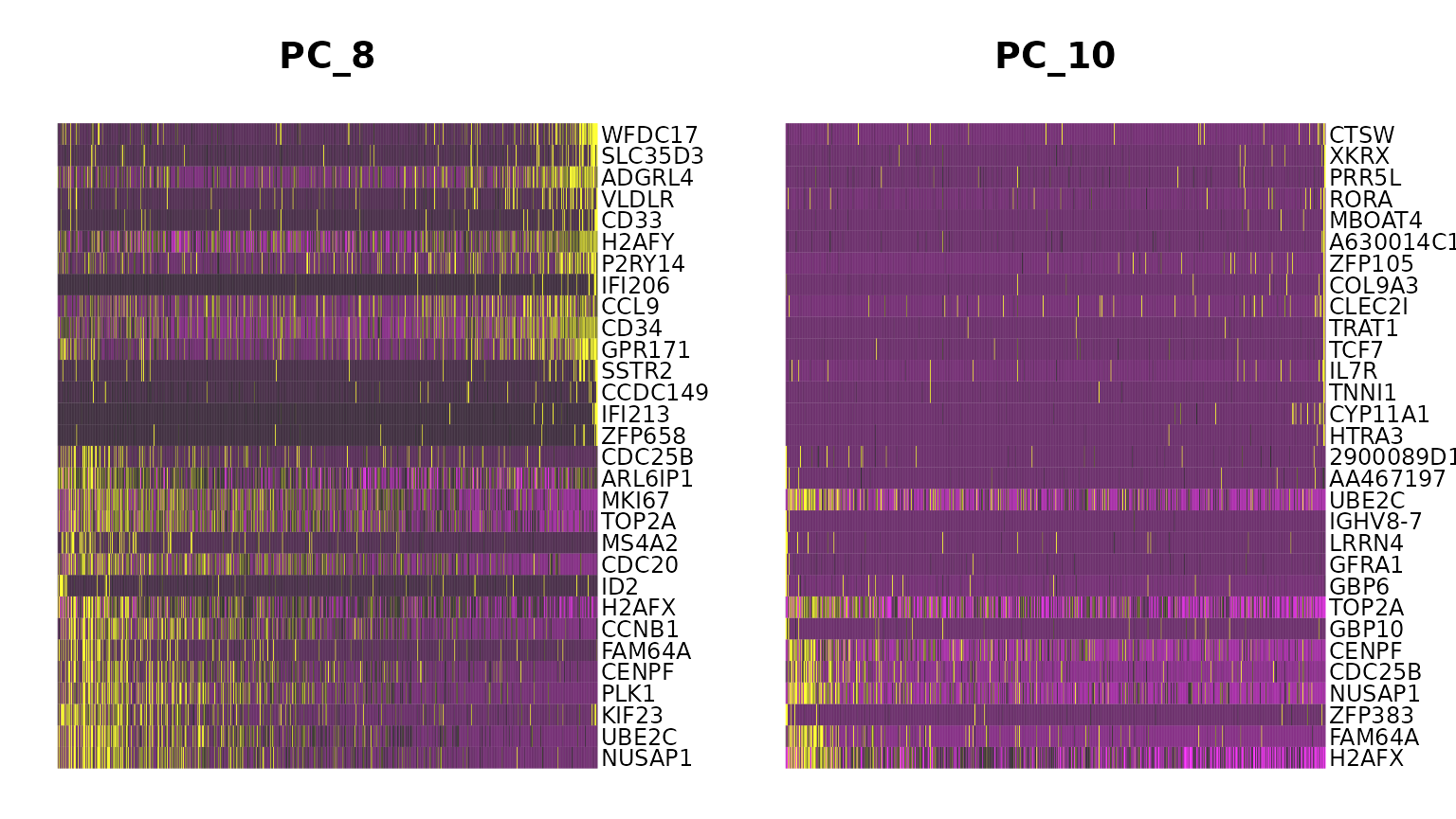
Assign Cell-Cycle Scores
First, we assign each cell a score, based on its expression of G2/M and S phase markers. These marker sets should be anticorrelated in their expression levels, and cells expressing neither are likely not cycling and in G1 phase.
We assign scores in the CellCycleScoring() function,
which stores S and G2/M scores in object meta data, along with the
predicted classification of each cell in either G2M, S or G1 phase.
CellCycleScoring() can also set the identity of the Seurat
object to the cell-cycle phase by passing set.ident = TRUE
(the original identities are stored as old.ident). Please
note that Seurat does not use the discrete classifications (G2M/G1/S) in
downstream cell cycle regression. Instead, it uses the quantitative
scores for G2M and S phase. However, we provide our predicted
classifications in case they are of interest.
marrow <- CellCycleScoring(marrow, s.features = s.genes, g2m.features = g2m.genes, set.ident = TRUE)

# View cell cycle scores and phase assignments
head(marrow[[]])
## orig.ident nCount_RNA nFeature_RNA S.Score G2M.Score Phase
## Prog_013 Prog 2563089 10211 -0.14248691 -0.4680395 G1
## Prog_019 Prog 3030620 9991 -0.16915786 0.5851766 G2M
## Prog_031 Prog 1293487 10192 -0.34627038 -0.3971879 G1
## Prog_037 Prog 1357987 9599 -0.44270212 0.6820229 G2M
## Prog_008 Prog 4079891 10540 0.55854051 0.1284359 S
## Prog_014 Prog 2569783 10788 0.07116218 0.3166073 G2M
## old.ident
## Prog_013 Prog
## Prog_019 Prog
## Prog_031 Prog
## Prog_037 Prog
## Prog_008 Prog
## Prog_014 Prog
# Visualize the distribution of cell cycle markers
RidgePlot(marrow, features = c("PCNA", "TOP2A", "MCM6", "MKI67"), ncol = 2)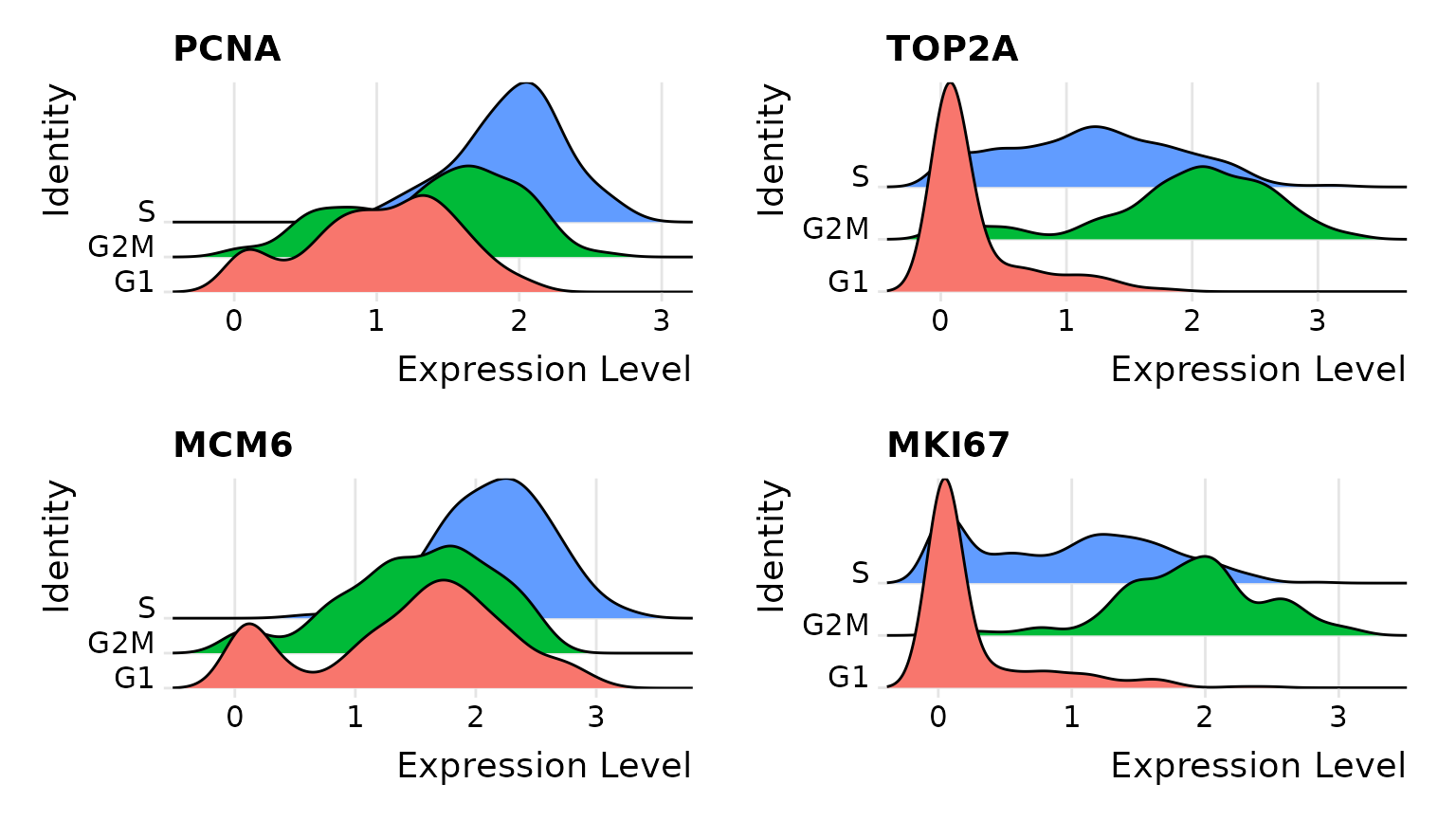
# Running a PCA on cell cycle genes reveals, unsurprisingly, that cells separate entirely by
# phase
marrow <- RunPCA(marrow, features = c(s.genes, g2m.genes))
DimPlot(marrow)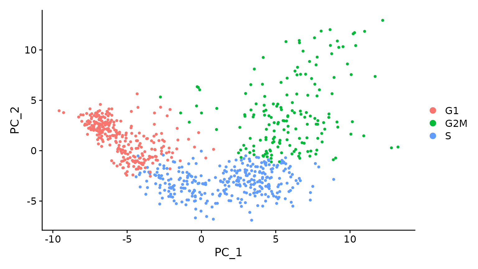
We score single cells based on the scoring strategy described in Tirosh et
al. 2016. See ?AddModuleScore() in Seurat for more
information, this function can be used to calculate supervised module
scores for any gene list.
Regress out cell cycle scores during data scaling
We now attempt to subtract (‘regress out’) this source of
heterogeneity from the data. For users of Seurat v1.4, this was
implemented in RegressOut. However, as the results of this
procedure are stored in the scaled data slot (therefore overwriting the
output of ScaleData()), we now merge this functionality
into the ScaleData() function itself.
For each gene, Seurat models the relationship between gene expression and the S and G2M cell cycle scores. The scaled residuals of this model represent a ‘corrected’ expression matrix, that can be used downstream for dimensional reduction.
marrow <- ScaleData(marrow, vars.to.regress = c("S.Score", "G2M.Score"), features = rownames(marrow))
# Now, a PCA on the variable genes no longer returns components associated with cell cycle
marrow <- RunPCA(marrow, features = VariableFeatures(marrow), nfeatures.print = 10)
## PC_ 1
## Positive: BLVRB, CAR2, KLF1, AQP1, CES2G, ERMAP, CAR1, FAM132A, RHD, SPHK1
## Negative: TMSB4X, H2AFY, CORO1A, PLAC8, EMB, MPO, PRTN3, CD34, LCP1, BC035044
## PC_ 2
## Positive: ANGPT1, ADGRG1, MEIS1, ITGA2B, MPL, DAPP1, APOE, RAB37, GATA2, F2R
## Negative: LY6C2, ELANE, HP, IGSF6, ANXA3, CTSG, CLEC12A, TIFAB, SLPI, ALAS1
## PC_ 3
## Positive: APOE, GATA2, NKG7, MUC13, MS4A3, RAB44, HDC, CPA3, FCGR3, TUBA8
## Negative: FLT3, DNTT, LSP1, WFDC17, MYL10, GIMAP6, LAX1, GPR171, TBXA2R, SATB1
## PC_ 4
## Positive: CSRP3, ST8SIA6, DNTT, MPEG1, SCIN, LGALS1, CMAH, RGL1, APOE, MFSD2B
## Negative: PROCR, MPL, HLF, MMRN1, SERPINA3G, ESAM, GSTM1, D630039A03RIK, MYL10, LY6A
## PC_ 5
## Positive: CPA3, LMO4, IKZF2, IFITM1, FUT8, MS4A2, SIGLECF, CSRP3, HDC, RAB44
## Negative: PF4, GP1BB, SDPR, F2RL2, RAB27B, SLC14A1, TREML1, PBX1, F2R, TUBA8
# When running a PCA on only cell cycle genes, cells no longer separate by cell-cycle phase
marrow <- RunPCA(marrow, features = c(s.genes, g2m.genes))
DimPlot(marrow)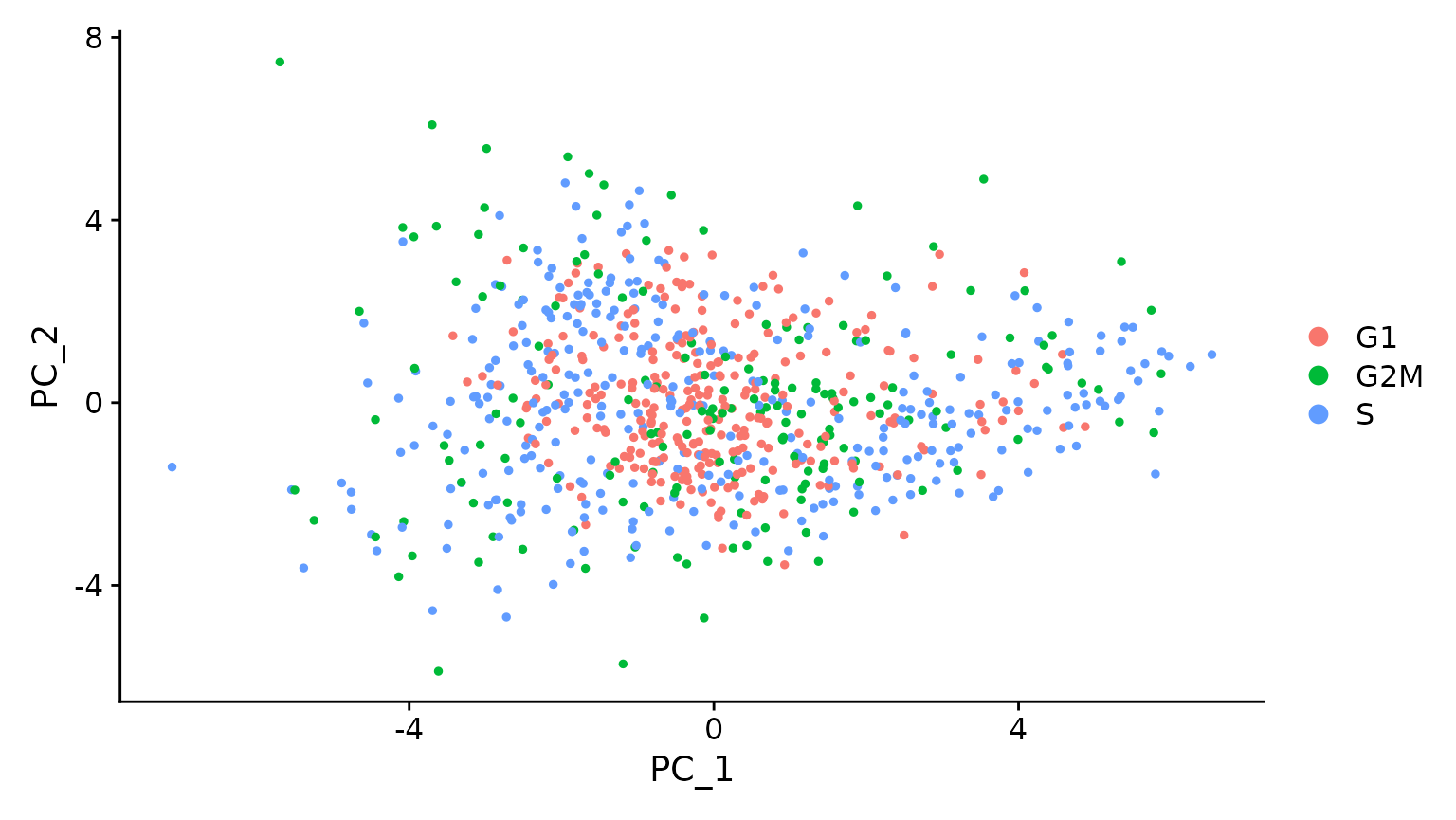
As the best cell cycle markers are extremely well conserved across tissues and species, we have found this procedure to work robustly and reliably on diverse datasets.
Alternate Workflow
The procedure above removes all signal associated with cell cycle. In some cases, we’ve found that this can negatively impact downstream analysis, particularly in differentiating processes (like murine hematopoiesis), where stem cells are quiescent and differentiated cells are proliferating (or vice versa). In this case, regressing out all cell cycle effects can blur the distinction between stem and progenitor cells as well.
As an alternative, we suggest regressing out the difference between the G2M and S phase scores. This means that signals separating non-cycling cells and cycling cells will be maintained, but differences in cell cycle phase among proliferating cells (which are often uninteresting), will be regressed out of the data
marrow$CC.Difference <- marrow$S.Score - marrow$G2M.Score
marrow <- ScaleData(marrow, vars.to.regress = "CC.Difference", features = rownames(marrow))
# cell cycle effects strongly mitigated in PCA
marrow <- RunPCA(marrow, features = VariableFeatures(marrow), nfeatures.print = 10)
## PC_ 1
## Positive: BLVRB, KLF1, ERMAP, FAM132A, CAR2, RHD, CES2G, SPHK1, AQP1, SLC38A5
## Negative: TMSB4X, CORO1A, PLAC8, H2AFY, LAPTM5, CD34, LCP1, TMEM176B, IGFBP4, EMB
## PC_ 2
## Positive: APOE, GATA2, RAB37, ANGPT1, ADGRG1, MEIS1, MPL, F2R, PDZK1IP1, DAPP1
## Negative: CTSG, ELANE, LY6C2, HP, CLEC12A, ANXA3, IGSF6, TIFAB, SLPI, MPO
## PC_ 3
## Positive: APOE, GATA2, NKG7, MUC13, ITGA2B, TUBA8, CPA3, RAB44, SLC18A2, CD9
## Negative: DNTT, FLT3, WFDC17, LSP1, MYL10, LAX1, GIMAP6, IGHM, CD24A, MN1
## PC_ 4
## Positive: CSRP3, ST8SIA6, SCIN, LGALS1, APOE, ITGB7, MFSD2B, RGL1, DNTT, IGHV1-23
## Negative: MPL, MMRN1, PROCR, HLF, SERPINA3G, ESAM, PTGS1, D630039A03RIK, NDN, PPIC
## PC_ 5
## Positive: GP1BB, PF4, SDPR, F2RL2, TREML1, RAB27B, SLC14A1, PBX1, PLEK, TUBA8
## Negative: HDC, LMO4, CSRP3, IFITM1, FCGR3, HLF, CPA3, PROCR, PGLYRP1, IKZF2
# when running a PCA on cell cycle genes, actively proliferating cells remain distinct from G1
# cells however, within actively proliferating cells, G2M and S phase cells group together
marrow <- RunPCA(marrow, features = c(s.genes, g2m.genes))
DimPlot(marrow)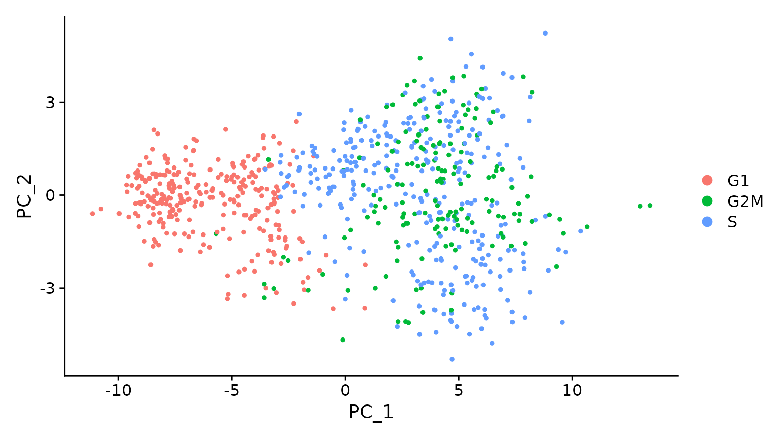
Session Info
## R version 4.5.2 (2025-10-31)
## Platform: x86_64-pc-linux-gnu
## Running under: Ubuntu 24.04.4 LTS
##
## Matrix products: default
## BLAS:   /usr/lib/x86_64-linux-gnu/openblas-pthread/libblas.so.3
## LAPACK: /usr/lib/x86_64-linux-gnu/openblas-pthread/libopenblasp-r0.3.26.so;  LAPACK version 3.12.0
##
## locale:
##  [1] LC_CTYPE=en_US.UTF-8       LC_NUMERIC=C
##  [3] LC_TIME=en_US.UTF-8        LC_COLLATE=en_US.UTF-8
##  [5] LC_MONETARY=en_US.UTF-8    LC_MESSAGES=en_US.UTF-8
##  [7] LC_PAPER=en_US.UTF-8       LC_NAME=C
##  [9] LC_ADDRESS=C               LC_TELEPHONE=C
## [11] LC_MEASUREMENT=en_US.UTF-8 LC_IDENTIFICATION=C
##
## time zone: Etc/UTC
## tzcode source: system (glibc)
##
## attached base packages:
## [1] stats     graphics  grDevices utils     datasets  methods   base
##
## other attached packages:
## [1] ggplot2_4.0.3      Seurat_5.5.0       SeuratObject_5.4.0 sp_2.2-1
##
## loaded via a namespace (and not attached):
##   [1] RColorBrewer_1.1-3     jsonlite_2.0.0         magrittr_2.0.5
##   [4] spatstat.utils_3.2-2   ggbeeswarm_0.7.3       farver_2.1.2
##   [7] rmarkdown_2.30         fs_2.1.0               ragg_1.5.1
##  [10] vctrs_0.7.1            ROCR_1.0-12            spatstat.explore_3.8-0
##  [13] htmltools_0.5.9        sass_0.4.10            sctransform_0.4.3
##  [16] parallelly_1.47.0      KernSmooth_2.23-26     bslib_0.10.0
##  [19] htmlwidgets_1.6.4      desc_1.4.3             ica_1.0-3
##  [22] plyr_1.8.9             plotly_4.12.0          zoo_1.8-15
##  [25] cachem_1.1.0           igraph_2.3.0           mime_0.13
##  [28] lifecycle_1.0.5        pkgconfig_2.0.3        Matrix_1.7-5
##  [31] R6_2.6.1               fastmap_1.2.0          fitdistrplus_1.2-6
##  [34] future_1.70.0          shiny_1.13.0           digest_0.6.39
##  [37] patchwork_1.3.2        tensor_1.5.1           RSpectra_0.16-2
##  [40] irlba_2.3.7            textshaping_1.0.5      labeling_0.4.3
##  [43] progressr_0.19.0       spatstat.sparse_3.1-0  httr_1.4.8
##  [46] polyclip_1.10-7        abind_1.4-8            compiler_4.5.2
##  [49] withr_3.0.2            S7_0.2.1               fastDummies_1.7.6
##  [52] MASS_7.3-65            tools_4.5.2            vipor_0.4.7
##  [55] lmtest_0.9-40          otel_0.2.0             beeswarm_0.4.0
##  [58] httpuv_1.6.16          future.apply_1.20.2    goftest_1.2-3
##  [61] glue_1.8.0             nlme_3.1-168           promises_1.5.0
##  [64] grid_4.5.2             Rtsne_0.17             cluster_2.1.8.2
##  [67] reshape2_1.4.5         generics_0.1.4         gtable_0.3.6
##  [70] spatstat.data_3.1-9    tidyr_1.3.2            data.table_1.18.2.1
##  [73] spatstat.geom_3.7-3    RcppAnnoy_0.0.23       ggrepel_0.9.8
##  [76] RANN_2.6.2             pillar_1.11.1          stringr_1.6.0
##  [79] spam_2.11-3            RcppHNSW_0.6.0         later_1.4.8
##  [82] splines_4.5.2          dplyr_1.2.0            lattice_0.22-7
##  [85] survival_3.8-3         deldir_2.0-4           tidyselect_1.2.1
##  [88] miniUI_0.1.2           pbapply_1.7-4          knitr_1.51
##  [91] gridExtra_2.3          scattermore_1.2        xfun_0.56
##  [94] matrixStats_1.5.0      stringi_1.8.7          lazyeval_0.2.3
##  [97] yaml_2.3.12            evaluate_1.0.5         codetools_0.2-20
## [100] tibble_3.3.1           cli_3.6.6              uwot_0.2.4
## [103] xtable_1.8-8           reticulate_1.46.0      systemfonts_1.3.2
## [106] jquerylib_0.1.4        Rcpp_1.1.1-1.1         globals_0.19.1
## [109] spatstat.random_3.4-5  png_0.1-9              ggrastr_1.0.2
## [112] spatstat.univar_3.1-7  parallel_4.5.2         pkgdown_2.2.0
## [115] dotCall64_1.2          listenv_0.10.1         viridisLite_0.4.3
## [118] scales_1.4.0           ggridges_0.5.7         purrr_1.2.1
## [121] rlang_1.2.0            cowplot_1.2.0          formatR_1.14