scSLIDE for single-cell sample-level analysis

Introduction

This vignette walks you through our Single-cell Sample-Level Inference using Density Estimation (scSLIDE) workflow, a computational method that performs sample-level analysis for single-cell data. Given a multi-sample single-cell dataset, scSLIDE first constructs a cell-type-oriented embedding (via reference mapping, integration, or unsupervised dimension reduction) and a disease-oriented embedding (via a supervised learning method, partial least squares, PLS). It then combines these two embeddings into a joint WNN embedding, placing cells in a joint space where their distances reflect both cell-type and disease-state similarity. Next, we use a sketched subset of cells (called ‘landmarks’, originally proposed by Yi & Stanley) and quantify the cell density near each landmark for each sample. This produces a landmark-by-sample density matrix that quantitatively captures the similarities and differences among samples. Sample-level analyses such as clustering, pseudo-trajectory inference, and differential expression testing can then be performed on this sample-level embedding. The method is described by Jiang et al. (Cell, 2026).

The vignette has two parts:

Part 1 explains each step of the workflow using an in-memory subset (~104k cells) of a COVID-19 dataset.
Part 2 applies the workflow to a large on-disk dataset of Alzheimer’s disease (~1.4M cells) and focuses on what differs at this scale.

Setup and library loading

First, we load Seurat and the other packages necessary for this vignette. scSLIDE is available in Seurat v6.

for (package in c("Seurat", "princurve", "ggplot2", "ggridges")) {
  if (!requireNamespace(package, quietly = TRUE)) {
    install.packages(package)
  }
}

if (!requireNamespace("destiny", quietly = TRUE)) {
  BiocManager::install("destiny")
}

if (!requireNamespace("BPCells", quietly = TRUE)) {
  remotes::install_github("bnprks/BPCells/r")
}
library(Seurat)
library(BPCells)
library(princurve)
library(ggplot2)
library(ggridges)

Part 1: Quick start with a COVID-19 dataset

Data loading and initial processing

For demonstration, we use a subset (~104k cells) of a COVID-19 dataset generated by Ahern et al 2022 Cell. This subset can be downloaded from this link. The dataset consists of 40 donors: 10 healthy controls (‘HV’) and 10 patients from each of 3 COVID severity groups (“MILD”, “SEV”, “CRIT”).

object <- readRDS("Raw_count_Subset_104k_Ahern_2022_Cell.rds")

# standard normalization
object <- NormalizeData(object)

Cell type annotation with Azimuth

We use the Pan-human Azimuth cloud tool to annotate our data and obtain a cell-type-oriented embedding. You can read more about this reference-mapping method in this paper. Note that you can instead use PCA or any other integration or reference-mapping method to obtain this embedding.

if (!requireNamespace("AzimuthAPI", quietly = TRUE)) {
  remotes::install_github("satijalab/AzimuthAPI")
}
library(AzimuthAPI)

object <- CloudAzimuth(object)

# get the top 2000 highly variable genes
object <- FindVariableFeatures(object, nfeatures = 2000)

Prepare the single-cell data for sample-level analysis

The wrapper function PrepareSampleObject() performs all the cell-level pre-processing steps required for sample-level embedding generation. It returns a Seurat object containing the landmark assay and a cell-to-landmark WNN graph, both of which are needed to generate the sample-level object.

object <- PrepareSampleObject(
  object = object,
  assay = "RNA",
  add.hvg = TRUE,
  group.by.CorTest = "azimuth_label",
  Y = "Disease",
  sketch.training = TRUE,
  group.by.Sketch = "Donor",
  ncells.per.group = 1000,
  ncells.landmark = 2000,
  ncomp = 20,
  pls.function = "cppls",
  k.nn = 5,
  name.reduction.1 = "azimuth_embed",
  dims.reduction.1 = 1:128,
  fix.wnn.weights = c(0.5, 0.5),
  verbose = TRUE)

What does PrepareSampleObject() actually do?

PrepareSampleObject() streamlines cell-level data preparation through the following steps:

Training subset creation (optional): Uses uniform sketching to obtain a training subset that balances the number of cells from each sample for PLS
Landmark cell selection: Uses leverage-score sketching to identify a diverse subset of landmark cells that captures the dataset’s heterogeneity
Disease-relevant gene selection (optional): Identifies additional highly variable genes associated with the phenotype of interest through correlation testing
Disease-oriented embedding: Runs PLS to generate an embedding that captures variation relevant to the specified response variable
Neighbor graph construction: Builds a weighted nearest neighbor (WNN) graph connecting landmark cells to all other cells in the dataset

For fine-grained control over individual parameters, the workflow below runs each of these steps manually.

Data sketching procedures

We sketch the data using two different procedures. The first draws a random subset of cells from each donor (e.g., n = 1000), so that the number of cells is approximately balanced across donors for supervised learning. This step is optional if the cell numbers are already balanced, but we recommend it for efficiency.

object <- SketchDataByGroup(
  object,
  assay = "RNA",
  ncells = 1000,
  sketched.assay = "TRAINING",
  method = "Uniform",
  group.by = "Donor",
  verbose = FALSE)

The second performs leverage-score sketching to select landmark cells that cover the diverse cell states in the data. We later generate the sample-level embedding using these landmarks.

object <- SketchData(
  object,
  assay = "TRAINING",
  ncells = 2000,
  sketched.assay = "LANDMARK",
  method = "LeverageScore",
  verbose = FALSE)

Disease-relevant gene selection

We can obtain additional disease-relevant genes to enhance PLS, in case the highly variable genes are not all relevant to the phenotype. If the variable features are already sufficiently informative, you can omit this step.

deg_list <- QuickCorTest(
  object,
  assay = "TRAINING",
  layer = "data",
  group.by = "azimuth_label",
  Y = "Disease",
  cor.cutoff = 0.2,
  verbose = FALSE)
all_HVG <- union(VariableFeatures(object), deg_list)

Supervised learning with partial least squares (PLS)

We apply PLS to the TRAINING data to obtain a disease-oriented low-dimensional embedding. RunPLS() supports three PLS algorithms: standard PLS (‘plsr’), canonical PLS (‘cppls’), and sparse PLS (‘spls’). Please see the RunPLS() manual for details.

DefaultAssay(object) <- "TRAINING"
object <- ScaleData(object, features = all_HVG)
object <- RunPLS(
  object = object,
  assay = "TRAINING",
  features = all_HVG,
  ncomp = 20,
  Y = c("Disease"),
  pls.function = "cppls",
  verbose = FALSE)

Projection to full dataset

We then project the learned PLS onto the full dataset and append the projected PLS embedding.

proj.pls <- ProjectCellEmbeddings(
  query = object,
  query.assay = "RNA",
  reference = object,
  reference.assay = "TRAINING",
  reduction = "pls",
  dims = 1:20,
  scale = TRUE,
  normalization.method = "LogNormalize",
  verbose = TRUE)

object[["proj.pls"]] <- CreateDimReducObject(
  embeddings = proj.pls,
  key = "pPLS_",
  assay = "RNA")
rm(proj.pls)
gc()

Joint embedding construction with weighted nearest neighbors

Having obtained the cell-type-oriented and disease-oriented embeddings, we generate a joint embedding that places cells in a space where distances reflect both types of information. We use the weighted nearest neighbor (WNN) procedure originally developed by Hao & Hao et al, Cell 2021, modified so that the modality weights of the two embeddings are both fixed at 0.5 and they contribute equally. You can set other values or let the algorithm learn the weights dynamically. The function returns a WNN graph between the landmark cells and all other cells in the dataset.

DefaultAssay(object) <- "RNA"

object <- FindmmNN(
  object,
  sketch.assay = "LANDMARK",
  reduction.list = list("azimuth_embed", "proj.pls"),
  k.nn = 5,
  nn.name = "weighted.nn",
  dims.list = list(1:128, 1:20),
  fix.wnn.weights = c(0.5, 0.5))

What if we only want to use a single modality to generate the NN graph?

By default, scSLIDE uses the WNN embedding to generate the sample-level embedding. To use a single modality instead (e.g., only the PLS embedding, or a custom embedding from another method), replace FindmmNN() with FindsmNN() and pass in that embedding. This returns a standard kNN graph that can be used directly for downstream sample-level embedding generation.

DefaultAssay(object) <- "RNA"

object <- FindsmNN(
  object,
  sketch.assay = "LANDMARK",
  reduction = "proj.pls",
  k.nn = 5,
  dims = 1:20,
  nn.name = "single.nn")

Click here to collapse ▲

Sample-level embedding generation

Once a WNN graph is constructed, we can generate a sample-level density matrix. Given the asymmetric landmark-by-cell WNN graph, scSLIDE aggregates over cells to obtain a landmark-by-sample density matrix (i.e., m landmarks by n samples) by binarizing adjacency (neighbor = 1, else 0) and summing per sample. Each entry in this matrix measures the cell density near a landmark for a given donor.

The function GenerateSampleObject() builds this sample-level object from the WNN graph specified by nn.name =. Optionally, it can also append donor-level metadata from the original single-cell object, and apply a Chi-squared normalization (based on the Poisson distribution of a contingency table) to the count matrix. Standard log-normalization is also supported.

sample_obj <- GenerateSampleObject(
  object = object,
  sketch.assay = "LANDMARK",
  nn.name = "weighted.nn",
  group.by = "Donor",
  rename.group.by = "azimuth_label",
  k.nn = 5,
  normalization.method = "ChiSquared",
  add.meta.data = TRUE,
  return.seurat = TRUE)

# center the data
sample_obj <- ScaleData(
  sample_obj,
  features = rownames(sample_obj),
  do.scale = FALSE,
  do.center = TRUE)

Diffusion map analysis

To better infer a trajectory from the sample-level data, we use Diffusion Map instead of standard PCA. Diffusion Map is a non-linear, unsupervised dimensional reduction method originally proposed by Haghverdi et al, Bioinformatics to capture single-cell trajectories.

sample_obj <- RunDiffusionMap(
  sample_obj,
  assay = "LMC",
  layer = "scale.data",
  features = rownames(sample_obj),
  ncomp = 10)

Visualizing the Diffusion Map components, we can see that DC1 captures case-control status, DC2 captures some COVID heterogeneity (not related to severity), and DC3 captures COVID severity.

DimPlot(sample_obj, reduction = "DiffMap", group.by = "Disease") +
  DimPlot(sample_obj, reduction = "DiffMap", group.by = "Disease", dims = c(1, 3))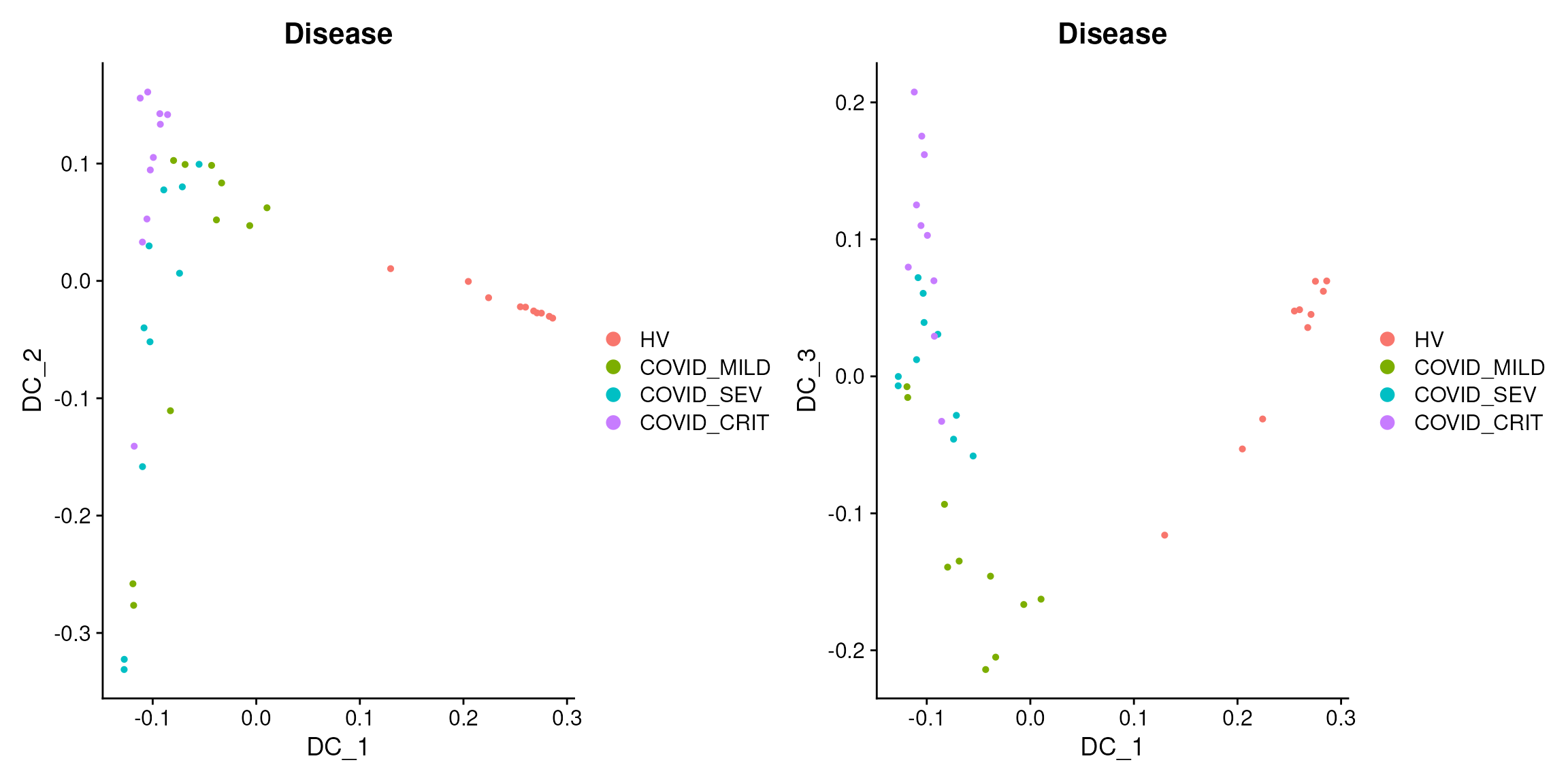

We append DC1-3 to the metadata and analyze their relationships with clinical variables.

sample_obj[["traj_DC1"]] <- sample_obj@reductions$DiffMap@cell.embeddings[, 1]
sample_obj[["traj_DC2"]] <- sample_obj@reductions$DiffMap@cell.embeddings[, 2]
sample_obj[["traj_DC3"]] <- sample_obj@reductions$DiffMap@cell.embeddings[, 3]

The following plots show that DC2 is related to TimeSinceOnset and DC3 is related to severity:

p1 <- FeatureScatter(
  sample_obj,
  feature1 = "traj_DC2",
  feature2 = "TimeSinceOnset",
  group.by = "Disease",
  cells = colnames(sample_obj)[sample_obj$Disease != "HV"],
  pt.size = 2)

p2 <- ggplot(sample_obj@meta.data[sample_obj$Disease != "HV", ]) +
  geom_density_ridges(aes(x = traj_DC3, y = Disease, fill = Disease), scale = 0.9) +
  theme_minimal() +
  theme(
    title = element_text(hjust = 0.5, size = 15),
    text = element_text(size = 13),
    axis.text.x = element_text(hjust = 1, vjust = 1, angle = 45),
    axis.text = element_text(size = 13))
print(p1 + p2)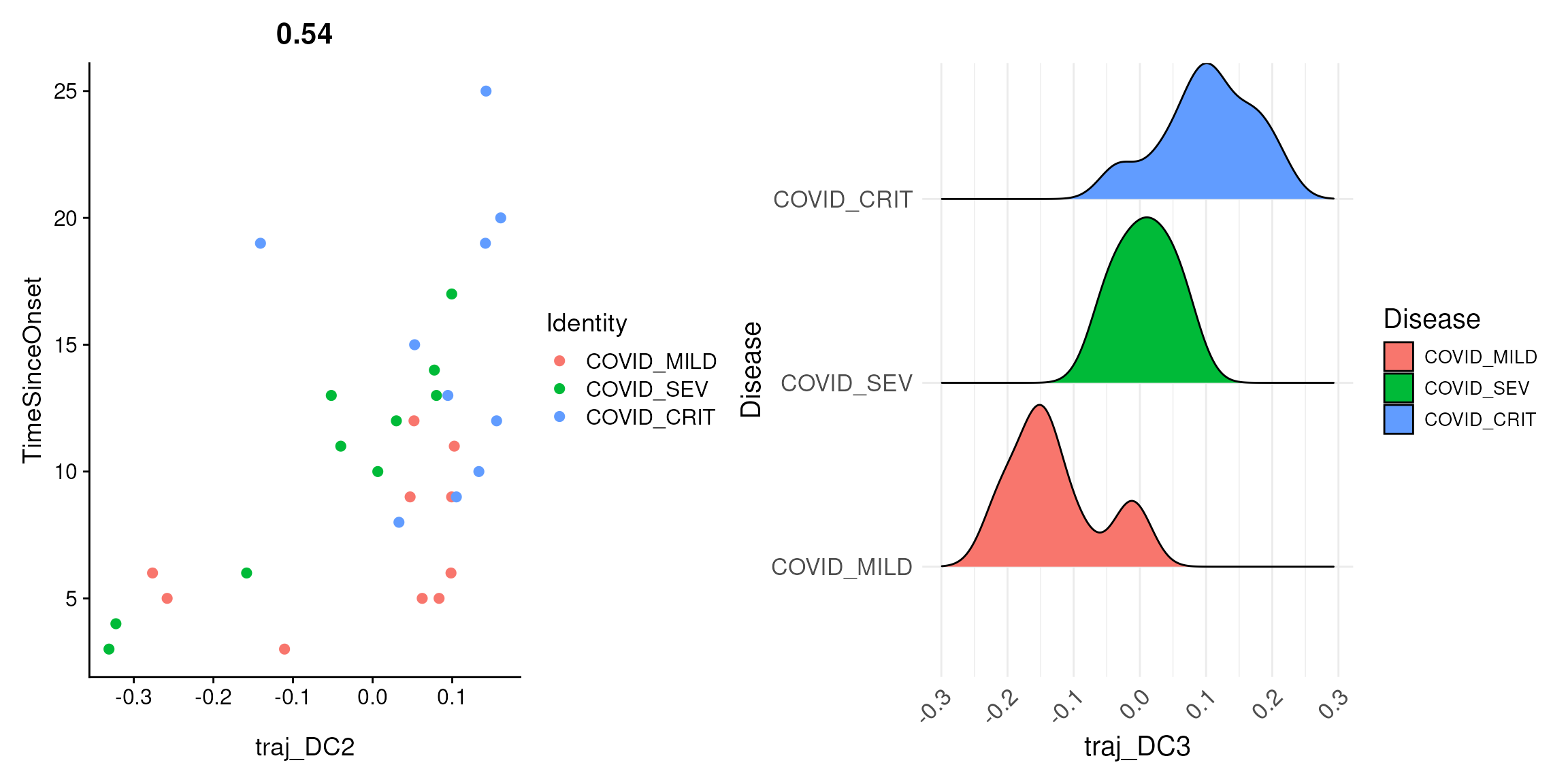

Fitting a joint pseudo-trajectory using a principal curve

Principal curve fitting

To explore whether multiple DCs can be merged, you can fit a principal curve to the top few DCs to obtain a single joint pseudo-trajectory. Here we fit a curve to the top 2 DCs and append it to the object.

princurve_res <- princurve::principal_curve(
  sample_obj[["DiffMap"]]@cell.embeddings[, 1:2],
  plot = FALSE,
  maxit = 20,
  trace = TRUE)
sample_obj[["traj_overall"]] <- princurve_res$lambda
DimPlot(sample_obj, reduction = "DiffMap", group.by = "Disease") +
  geom_path(aes(
    x = princurve_res$s[princurve_res$ord, 1],
    y = princurve_res$s[princurve_res$ord, 2]))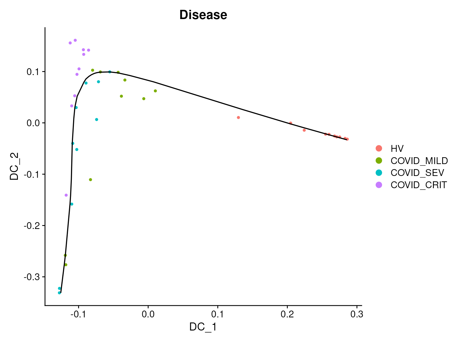

Differential expression analysis

Finally, we can perform differential expression (DE) analysis to identify differentially expressed genes (DEGs) along the inferred pseudo-trajectory. We test each DC separately, since we believe they represent distinct sources of biological variation.

First, we obtain the pseudobulk expression data from the original single-cell data:

bulk_obj <- AggregateExpression(
  object,
  assays = "RNA",
  group.by = c("Donor", "azimuth_label"),
  return.seurat = TRUE)

# append the metadata to the pseudobulk object
mdata <- object@meta.data[, c("Donor", "azimuth_label")]
mdata <- mdata[!duplicated(mdata), ]
rownames(mdata) <- paste0(
  gsub(pattern = "_", replacement = "-", mdata$Donor),
  "_",
  gsub(pattern = "_", replacement = "-", mdata$azimuth_label))
bulk_obj <- AddMetaData(bulk_obj, metadata = mdata)

bulk_obj$nCount_RNA <- colSums(x = bulk_obj, slot = "counts")
bulk_obj$nFeature_RNA <- colSums(x = LayerData(object = bulk_obj, layer = "counts") > 0)

DE analysis for CD14 monocytes

We run the DE analysis one cell type at a time, using CD14 monocytes as an example.

sub_bulk_obj <- subset(bulk_obj, subset = azimuth_label == "CD14 monocyte")

# add metadata from the sample-level object to the pseudobulk object
new_mdata <- merge(
  sub_bulk_obj@meta.data[, c("Donor"), drop = FALSE],
  sample_obj@meta.data[, c(
    "Donor", "Age", "Sex", "Disease", "traj_DC1", "traj_DC2", "traj_DC3")],
  by = "Donor",
  all.x = TRUE,
  sort = FALSE)
sub_bulk_obj <- AddMetaData(sub_bulk_obj, metadata = new_mdata)
sub_bulk_obj$log_count <- log10(sub_bulk_obj$nCount_RNA)

We can now run trajectory DE tests for DC1, DC2, and DC3. We remove healthy donors for DC2 and DC3 to concentrate on within-COVID heterogeneity.

# run the trajectory DE test for DC1
de_results <- TrajDETest(
  sub_bulk_obj,
  assay = "RNA",
  layer = "counts",
  traj.var = "traj_DC1",
  latent.vars = c("Age", "Sex", "log_count"))

# run the trajectory DE tests for DC2 and DC3
non_health_idx <- Cells(sub_bulk_obj)[sub_bulk_obj$Disease != "HV"]
de_results2 <- TrajDETest(
  sub_bulk_obj,
  assay = "RNA",
  layer = "counts",
  traj.var = "traj_DC2",
  latent.vars = c("Age", "Sex", "log_count"),
  samples = non_health_idx)

de_results3 <- TrajDETest(
  sub_bulk_obj,
  assay = "RNA",
  layer = "counts",
  traj.var = "traj_DC3",
  latent.vars = c("Age", "Sex", "log_count"),
  samples = non_health_idx)

From the DE results, we identify the top up- and down-regulated DEGs for visualization:

de_results$sign <- sign(de_results$beta_Traj)
de_results <- de_results[order(de_results$sign, de_results$p_Traj), ]
DEG_DC1 <- c(
  de_results$gene_ID[de_results$sign > 0][1:20],
  de_results$gene_ID[de_results$sign < 0][20:1])

de_results2$sign <- sign(de_results2$beta_Traj)
de_results2 <- de_results2[order(de_results2$sign, de_results2$p_Traj), ]
DEG_DC2 <- c(
  de_results2$gene_ID[de_results2$sign > 0][1:20],
  de_results2$gene_ID[de_results2$sign < 0][20:1])

de_results3$sign <- sign(de_results3$beta_Traj)
de_results3 <- de_results3[order(de_results3$sign, de_results3$p_Traj), ]
DEG_DC3 <- c(
  de_results3$gene_ID[de_results3$sign > 0][1:20],
  de_results3$gene_ID[de_results3$sign < 0][20:1])

The visualization function PlotAnnotatedHeatmap() (which adopts the style and color scheme of Scillus, a package that is no longer maintained for Seurat > v5.3) generates a pseudobulk heatmap. Here is the heatmap for DC1, with donors ordered by DC1:

sub_bulk_obj <- ScaleData(sub_bulk_obj, features = DEG_DC1)

PlotAnnotatedHeatmap(
  object = sub_bulk_obj,
  features = DEG_DC1,
  sort.by = "traj_DC1",
  anno.var = "Disease",
  anno.colors = list(c("#f8766d", "cornsilk", "#7cae02", "blue1", "#01bfc4", "#c77cff")),
  hm.colors = c("blue", "white", "red"))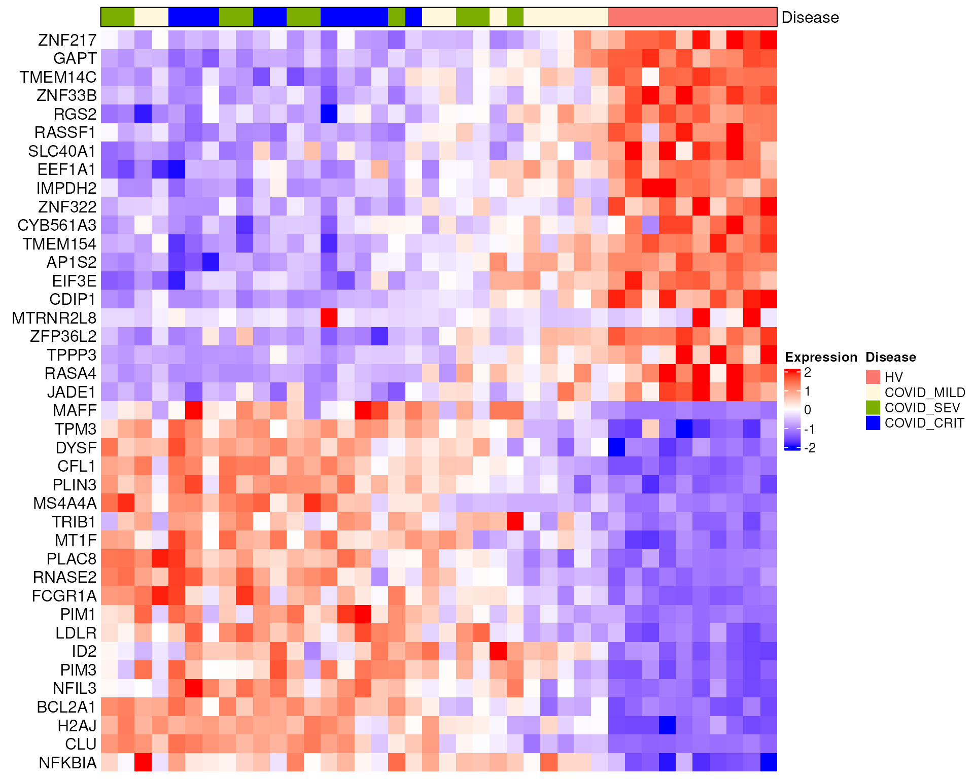

Here are the heatmaps for DC2 and DC3, with healthy donors removed:

sub_bulk_obj2 <- subset(sub_bulk_obj, cells = non_health_idx)
sub_bulk_obj2 <- ScaleData(sub_bulk_obj2, features = c(DEG_DC1, DEG_DC2, DEG_DC3))

PlotAnnotatedHeatmap(
  object = sub_bulk_obj2,
  features = DEG_DC2,
  sort.by = "traj_DC2",
  anno.var = "Disease",
  anno.colors = list(c("cornsilk", "#7cae02", "blue1", "#01bfc4", "#c77cff")),
  hm.colors = c("blue", "white", "red"))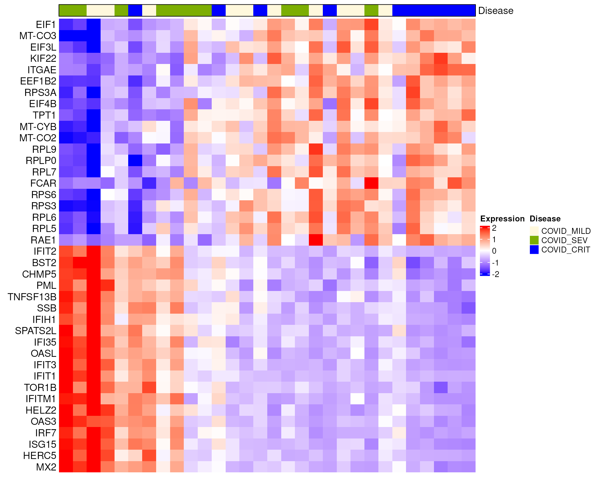

PlotAnnotatedHeatmap(
  object = sub_bulk_obj2,
  features = DEG_DC3,
  sort.by = "traj_DC3",
  anno.var = "Disease",
  anno.colors = list(c("cornsilk", "#7cae02", "blue1", "#01bfc4", "#c77cff")),
  hm.colors = c("blue", "white", "red"))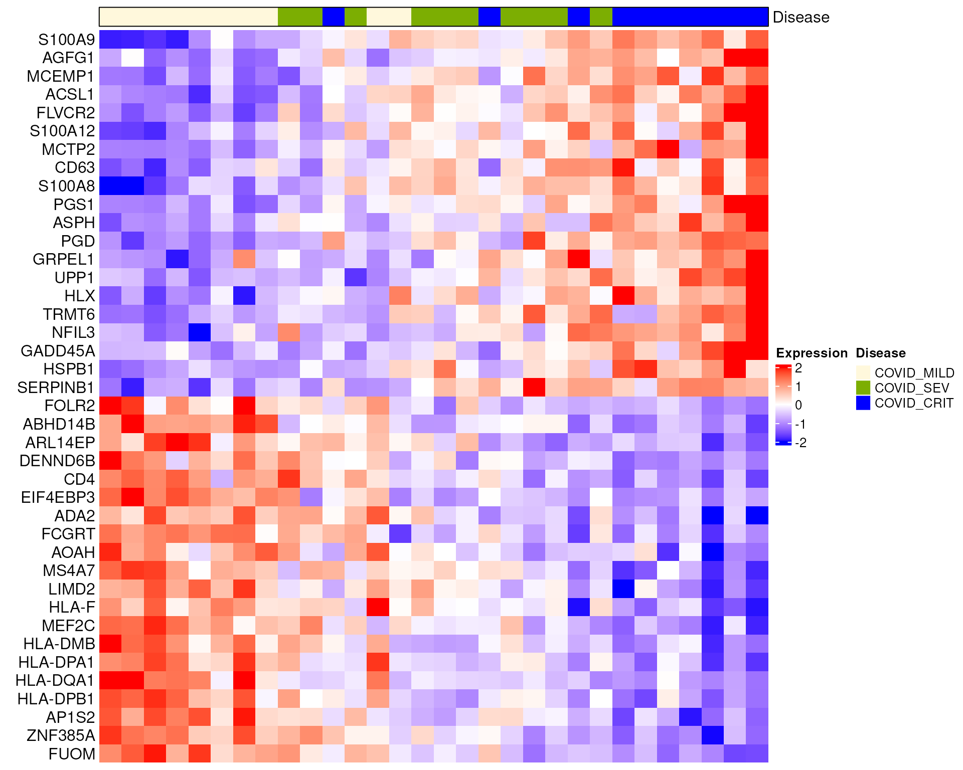

Part 2: On-disk analysis of a large-scale AD dataset

This part demonstrates scSLIDE on a large-scale dataset using the Seurat–BPCells infrastructure. Developed by Benjamin Parks, BPCells enables efficient storage and processing of large scRNA-seq and scATAC-seq datasets while minimizing memory usage. The workflow follows Part 1, so we focus here on what differs.

# dataset name used in the file paths below
DATA_NAME <- "SEA_AD_atlas_MTG"

Generating an on-disk Seurat object from an .h5ad file

We use the SEA-AD single-nucleus RNA-seq (snRNA-seq) data (~1.4M cells) of Alzheimer’s disease from the Allen Institute, published by Gabitto et al 2024 Nat. Neurosci.. This dataset can be downloaded from the CZI CELLxGENE data portal. Several datasets are available at this link; we use the data collected from the patients’ MTG (middle temporal gyrus) region.

The original file is in the .h5ad AnnData format. You can load the whole dataset into R using packages such as the anndata R package, but this is often not memory-efficient. Below, we show how to generate an on-disk Seurat object from the .h5ad file, which we then use for our scSLIDE analysis.

If your data does not contain cell-type labels or has not been properly integrated, you may want to first annotate your .h5ad file using our Pan-Human Azimuth Python tool. It annotates your cells and also computes a cell-type-oriented low-dimensional embedding for them. You can do this by following these simple instructions.

Click here to see how to generate an on-disk Seurat object from the SEA-AD .h5ad file

# path to the h5ad file (assuming it has been annotated by the Pan-Human Azimuth Python tool)
file_path <- "./SEA_AD_atlas_MTG_ANN.h5ad"

# path to save the on-disk matrix (from BPCells)
ondisk_path <- paste0("./", DATA_NAME, "_ondisk/")

# load the count matrix with BPCells
ondisk.data <- open_matrix_anndata_hdf5(file_path, group = "/X")
# write this BPCells matrix to disk
write_matrix_dir(mat = ondisk.data, dir = ondisk_path)

# get the necessary components from the original h5ad file
if (!requireNamespace("schard", quietly = TRUE)) {
  remotes::install_github("cellgeni/schard")
}

# feature names
feature_metadata <- schard::h5ad2data.frame(file_path, "var")
# metadata
metadata <- schard::h5ad2data.frame(file_path, "obs")
# Pan-Human Azimuth embedding
ann_embedding <- t(schard::h5ad2Matrix(file_path, "/obsm/azimuth_embed"))

# load the on-disk BPCells data
ondisk.mat <- open_matrix_dir(dir = ondisk_path)

# rename the features using gene symbols instead of ENSG IDs
rownames(ondisk.mat) <- feature_metadata$feature_name

# create an on-disk Seurat object with the metadata; it links to the `ondisk.mat` matrix
ondisk.object <- CreateSeuratObject(counts = ondisk.mat, meta.data = metadata)

# add the Azimuth embedding to the Seurat object
rownames(ann_embedding) <- colnames(ondisk.object)
ondisk.object[["azimuth_embed"]] <- CreateDimReducObject(
  embeddings = ann_embedding,
  assay = "RNA",
  key = "Ann_")

# basic QC: filter on nCount and nFeature
ondisk.object <- subset(ondisk.object, subset = nCount_RNA >= 1000 & nFeature_RNA >= 500)
# remove cells with discordant cell-type labels
ondisk.object <- subset(ondisk.object, subset = full_consistent_hierarchy == TRUE)
# remove cells with a very low final-level probability
ondisk.object <- subset(ondisk.object, subset = final_level_softmax_prob >= 0.6)

# remove cell types with fewer than 50 cells
ct_table <- table(ondisk.object$Subclass)
keep_celltype <- names(ct_table)[ct_table >= 50]
ondisk.object <- subset(ondisk.object, subset = Subclass %in% keep_celltype)

# generate the necessary metadata columns
ondisk.object$Donor <- as.character(ondisk.object$donor_id)
ondisk.object$dementia <- ondisk.object$disease
# recode disease status as HV or AD
ondisk.object$Disease <- "HV"
ondisk.object$Disease[!ondisk.object$ADNC %in% c("Not AD", "Reference")] <- "AD"
ondisk.object$Disease <- factor(ondisk.object$Disease, levels = c("HV", "AD"))

# fix the Age and Sex metadata
ondisk.object$Sex <- ondisk.object$sex
# donors labelled "80 year-old and over human stage" are actually >= 90 years old
# (the label is inconsistent with 'Age at death'), so we fix this manually
ondisk.object$Age <- gsub(
  pattern = "-year-old human stage",
  replacement = "",
  ondisk.object$development_stage)
ondisk.object$Age[ondisk.object$development_stage == "80 year-old and over human stage"] <- 90
ondisk.object$Age <- as.numeric(ondisk.object$Age)

# save the object for later use
saveRDS(ondisk.object, file = paste0("Seurat_obj_1_OnDisk_", DATA_NAME, ".rds"))
rm(ondisk.object, ann_embedding, metadata, feature_metadata, ondisk.mat, ondisk.data)
gc()

Click here to collapse ▲

Loading and preprocessing the on-disk data

We load the on-disk Seurat object into R and process it just like a regular in-memory object, running normalization and variable feature selection.

# load the on-disk Seurat object
object <- readRDS(paste0("./Seurat_obj_1_OnDisk_", DATA_NAME, ".rds"))

# basic processing
object <- NormalizeData(object)
object <- FindVariableFeatures(object, nfeatures = 3000)

Prepare the single-cell data for sample-level analysis

We run the same PrepareSampleObject() wrapper as in Part 1, where you can read how to break it down into individual steps.

Here we use setThreads() for parallelization to reduce the runtime, requesting 8 cores. Note that setThreads() is now supported by other core functions in Seurat (version >= 5.6).

setThreads(n = 8)

object <- PrepareSampleObject(
  object = object,
  assay = "RNA",
  add.hvg = TRUE,
  group.by.CorTest = "Subclass",
  Y = "Disease",
  sketch.training = TRUE,
  group.by.Sketch = "Donor",
  ncells.per.group = 3000,
  ncells.landmark = 5000,
  ncomp = 20,
  pls.function = "cppls",
  k.nn = 5,
  name.reduction.1 = "azimuth_embed",
  dims.reduction.1 = 1:128,
  fix.wnn.weights = c(0.5, 0.5),
  rm.training.assay = TRUE,
  verbose = TRUE)

Sample-level embedding generation

We generate the sample-level object as described in Part 1. One additional step here is to filter out donors with few cells.

sample_obj <- GenerateSampleObject(
  object = object,
  sketch.assay = "LANDMARK",
  nn.name = "weighted.nn",
  group.by = "Donor",
  rename.group.by = "Subclass",
  k.nn = 5,
  normalization.method = "ChiSquared",
  add.meta.data = TRUE,
  return.seurat = TRUE,
  new_assay_name = "LMC")

# filter out donors with fewer than 200 cells (i.e., nCount_LMC = k.nn * cell_count < 1000)
sample_obj <- subset(sample_obj, subset = nCount_LMC >= 1000)

# center the data
sample_obj <- ScaleData(
  sample_obj,
  features = rownames(sample_obj),
  do.scale = FALSE,
  do.center = TRUE)

Diffusion map analysis

As in Part 1, we run Diffusion Map on the sample-level data.

sample_obj <- RunDiffusionMap(
  sample_obj,
  assay = "LMC",
  layer = "scale.data",
  features = rownames(sample_obj),
  ncomp = 5)

Visualizing the Diffusion Map components, we can see what appears to be a progression trajectory jointly captured by DC1 and DC2.

DimPlot(sample_obj, reduction = "DiffMap", group.by = "Disease")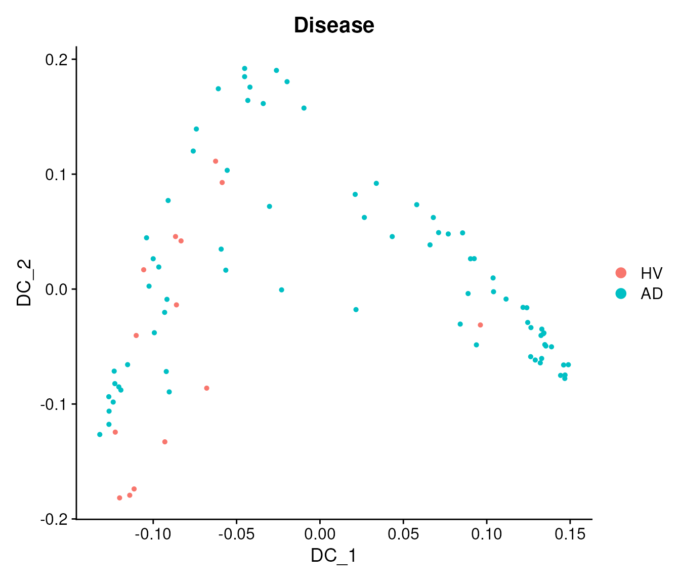

We append DC1-3 to the metadata.

sample_obj[["traj_DC1"]] <- sample_obj@reductions$DiffMap@cell.embeddings[, 1]
sample_obj[["traj_DC2"]] <- sample_obj@reductions$DiffMap@cell.embeddings[, 2]
sample_obj[["traj_DC3"]] <- sample_obj@reductions$DiffMap@cell.embeddings[, 3]

Principal curve fitting

Because the first two DCs appear to represent a joint trajectory, we fit a principal curve to them to infer a single pseudo-trajectory.

princurve_res <- princurve::principal_curve(
  sample_obj[["DiffMap"]]@cell.embeddings[, 1:2],
  plot = FALSE,
  maxit = 20,
  trace = TRUE)
sample_obj[["traj_overall"]] <- princurve_res$lambda
DimPlot(sample_obj, reduction = "DiffMap", group.by = "Disease") +
  geom_path(aes(
    x = princurve_res$s[princurve_res$ord, 1],
    y = princurve_res$s[princurve_res$ord, 2]))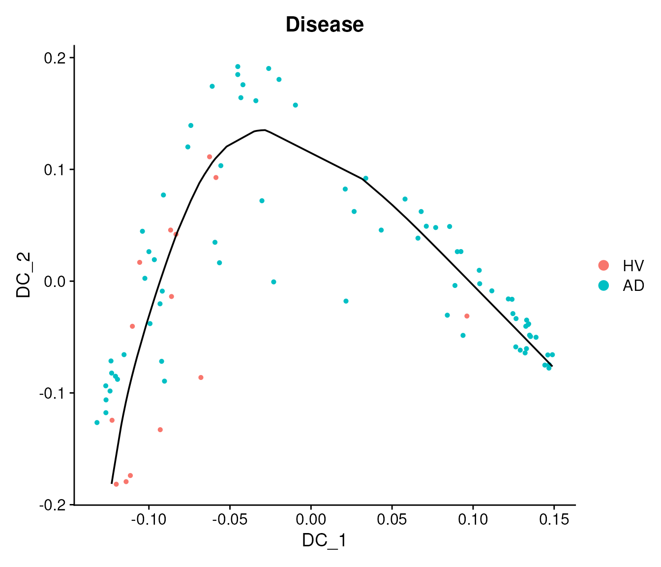

The following plot shows that the principal curve is related to the neuropathological continuous pseudo-progression score (CPS) provided by the original paper. The CPS values were obtained by aggregating various patient-level neuropathological measurements from postmortem brains, and are independent of the snRNA-seq data.

mdata <- sample_obj@meta.data
mdata$bin_traj_overall <- cut(
  rank(mdata$traj_overall),
  breaks = 5,
  labels = paste0("traj-bin_", 1:5))

p11 <- ggplot(data = mdata) +
  geom_boxplot(
    aes(x = bin_traj_overall, y = `Continuous Pseudo-progression Score`),
    outliers = FALSE) +
  geom_point(
    aes(
      x = bin_traj_overall,
      y = `Continuous Pseudo-progression Score`,
      col = Disease,
      shape = Disease),
    position = position_jitter(width = 0.2, height = 0)) +
  ggtitle("Pseudo-time vs. CPS") +
  theme_bw() +
  theme(
    title = element_text(hjust = 0.5, size = 15),
    text = element_text(size = 13),
    axis.text.x = element_text(hjust = 1, vjust = 1, angle = 45),
    axis.text = element_text(size = 13)) +
  xlab("Pseudo-trajectory bins") +
  ylab("Continuous Pseudo-progression Score")

print(p11)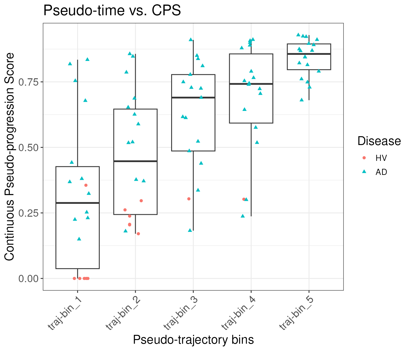

Differential expression analysis

As in Part 1, we perform DE analysis on pseudobulk data, but here we test the single joint pseudo-trajectory (traj_overall) rather than each DC separately.

First, we obtain the pseudobulk expression data from the original single-cell data:

bulk_obj <- AggregateExpression(
  object,
  assays = "RNA",
  group.by = c("Donor", "Subclass"),
  return.seurat = TRUE)

## Computing: [========================================] 100% (done)

# append the metadata to the pseudobulk object
mdata <- object@meta.data[, c("Donor", "Subclass")]
mdata <- mdata[!duplicated(mdata), ]
rownames(mdata) <- paste0(
  gsub(pattern = "_", replacement = "-", mdata$Donor),
  "_",
  gsub(pattern = "_", replacement = "-", mdata$Subclass))
bulk_obj <- AddMetaData(bulk_obj, metadata = mdata)

bulk_obj$nCount_RNA <- colSums(x = bulk_obj, slot = "counts")
bulk_obj$nFeature_RNA <- colSums(x = LayerData(object = bulk_obj, layer = "counts") > 0)

DE analysis for Microglia-PVM

We run the DE analysis one cell type at a time, using Microglia-PVM as an example.

sub_bulk_obj <- subset(bulk_obj, subset = Subclass == "Microglia-PVM")

# add metadata from the sample-level object to the pseudobulk object
new_mdata <- merge(
  sub_bulk_obj@meta.data[, c("Donor"), drop = FALSE],
  sample_obj@meta.data[, c("Donor", "Age", "Sex", "Disease", "traj_overall")],
  by = "Donor",
  all.x = TRUE,
  sort = FALSE)
sub_bulk_obj <- AddMetaData(sub_bulk_obj, metadata = new_mdata)
sub_bulk_obj$log_count <- log10(sub_bulk_obj$nCount_RNA)

We can now run the trajectory DE test.

de_results <- TrajDETest(
  sub_bulk_obj,
  assay = "RNA",
  layer = "counts",
  traj.var = "traj_overall",
  latent.vars = c("Age", "Sex", "log_count"))

From the DE results, we identify the top up- and down-regulated DEGs for visualization, omitting genes with MT- or RP prefixes:

de_results$sign <- sign(de_results$beta_Traj)
de_results <- de_results[order(de_results$sign, de_results$p_Traj), ]

# omit genes with MT- or RP prefixes for visualization
de_results <- de_results[!grepl("^(MT-|RP)", de_results$gene_ID), ]

DEG_traj_overall <- c(
  de_results$gene_ID[de_results$sign > 0][1:20],
  de_results$gene_ID[de_results$sign < 0][20:1])

Here is the heatmap for traj_overall, with donors ordered by the trajectory:

sub_bulk_obj <- ScaleData(sub_bulk_obj, features = DEG_traj_overall)

PlotAnnotatedHeatmap(
  object = sub_bulk_obj,
  features = DEG_traj_overall,
  sort.by = "traj_overall",
  anno.var = "Disease",
  anno.colors = list(c("#f8766d", "cornsilk")),
  hm.colors = c("blue", "white", "red"))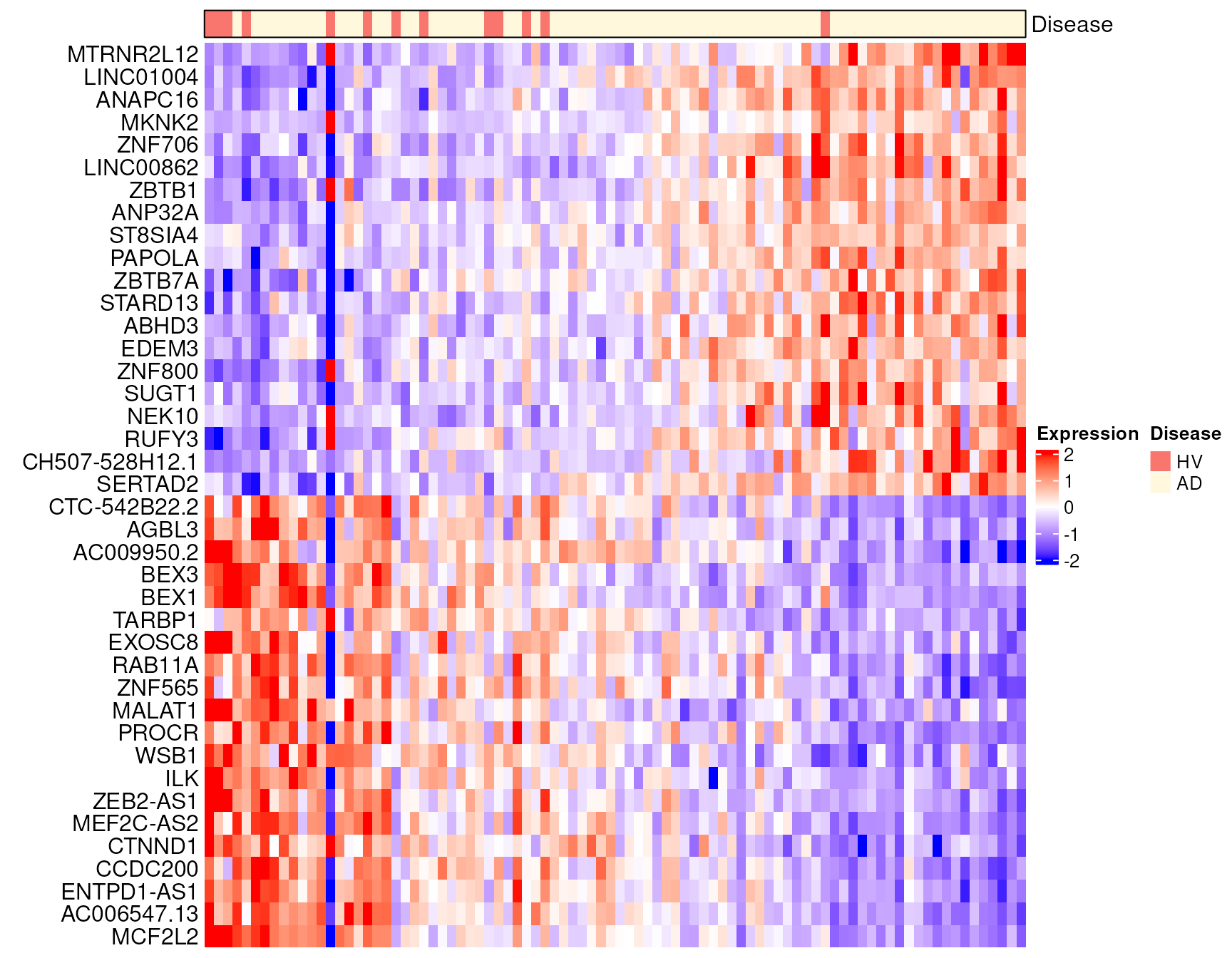

Session Info

sessioninfo::session_info(pkgs = "attached")

## ─ Session info ───────────────────────────────────────────────────────────────
##  setting  value
##  version  R version 4.5.2 (2025-10-31)
##  os       Ubuntu 24.04.4 LTS
##  system   x86_64, linux-gnu
##  ui       X11
##  language en
##  collate  en_US.UTF-8
##  ctype    en_US.UTF-8
##  tz       Etc/UTC
##  date     2026-11-06
##  pandoc   3.9 @ /usr/bin/ (via rmarkdown)
##  quarto   1.8.25 @ /usr/local/bin/quarto
## 
## ─ Packages ───────────────────────────────────────────────────────────────────
##  package      * version date (UTC) lib source
##  AzimuthAPI   * 1.0.1   2026-11-06 [3] Github (satijalab/AzimuthAPI@f08f243)
##  BPCells      * 0.3.1   2026-07-13 [3] https://b~
##  ggplot2      * 4.0.3   2026-04-22 [3] CRAN (R 4.5.2)
##  ggridges     * 0.5.7   2025-08-27 [3] CRAN (R 4.5.2)
##  princurve    * 2.1.6   2021-01-18 [3] RSPM (R 4.5.2)
##  Seurat       * 6.0.0   2026-11-06 [1] local
##  SeuratObject * 5.4.0   2026-04-11 [3] RSPM (R 4.5.0)
##  sp           * 2.2-4   2026-10-11 [3] RSPM (R 4.5.0)
## 
##  [1] /scratch/build-QLRyQPI9/library
##  [2] /usr/local/lib/R/custom-lib
##  [3] /usr/local/lib/R/site-library
##  [4] /usr/local/lib/R/library
##  * ── Packages attached to the search path.
## 
## ──────────────────────────────────────────────────────────────────────────────

Compiled: November 06, 2026

Introduction

Setup and library loading

Part 1: Quick start with a COVID-19 dataset

Data loading and initial processing

Cell type annotation with Azimuth

Prepare the single-cell data for sample-level analysis

Data sketching procedures

Disease-relevant gene selection

Supervised learning with partial least squares (PLS)

Projection to full dataset

Joint embedding construction with weighted nearest neighbors

What if we only want to use a single modality to generate the NN graph?

Sample-level embedding generation

Diffusion map analysis

Principal curve fitting

Differential expression analysis

DE analysis for CD14 monocytes

Part 2: On-disk analysis of a large-scale AD dataset

Generating an on-disk Seurat object from an .h5ad file

Loading and preprocessing the on-disk data

Prepare the single-cell data for sample-level analysis

Sample-level embedding generation

Diffusion map analysis

Principal curve fitting

Differential expression analysis

DE analysis for Microglia-PVM