Analyzing perturbation responses with RNA fingerprinting
Compiled: November 06, 2026
Source:vignettes/rna_fingerprinting.Rmd
rna_fingerprinting.RmdOverview
RNA fingerprinting (Grabski et al., Cell 2026) matches transcriptional responses to a dictionary of perturbation-specific expression patterns. In this vignette, we demonstrate RNA fingerprinting on a Perturb-seq dataset available on GEO under accession number GSE132080. Each targeted gene has five guide RNAs: one perfectly matched guide and four guides with nucleotide mismatches that titrate perturbation strength.
In this vignette, we first learn a dictionary from cells receiving perfectly matched guides and ask whether it can identify the perturbations in cells receiving mismatched guides. We then examine assignments at the gene, guide, and individual-cell levels to understand differences in perturbation strength and heterogeneity. Finally, we map the same dataset to precomputed Genome-Wide Perturb-seq (GWPS) fingerprints, extending the analysis to a larger reference without learning a new dictionary.
Analyzing a new experiment with RNA fingerprinting
Loading packages and preparing the data
We begin by loading the RNAFingerprinting
R package, Seurat, and other required packages. The final section also
requires the RNAFingerprintingData
companion package to access the precomputed GWPS dictionary.
Download GSE132080_10X_matrix.mtx.gz,
GSE132080_10X_barcodes.tsv.gz,
GSE132080_10X_genes.tsv.gz, and
GSE132080_cell_identities.csv.gz from GEO, and set
data_dir below to the directory containing these files. We
retain cells with a single-cell assignment and a known guide identity,
then extract the target gene and guide ID from the metadata.
if (!requireNamespace("RNAFingerprinting", quietly = TRUE)) {
  remotes::install_github("satijalab/rna-fingerprinting")
}
if (!requireNamespace("RNAFingerprintingData", quietly = TRUE)) {
  remotes::install_url("https://github.com/satijalab/rna-fingerprinting-data/raw/refs/heads/main/RNAFingerprintingData_0.1.0.tar.gz")
}
library(RNAFingerprinting)
library(RNAFingerprintingData)
library(Seurat)
library(pheatmap)
library(stringr)

data_dir <- "/brahms/grabskii/jost_data"

counts <- ReadMtx(mtx = file.path(data_dir, "GSE132080_10X_matrix.mtx.gz"),
                  cells = file.path(data_dir, "GSE132080_10X_barcodes.tsv.gz"),
                  features = file.path(data_dir, "GSE132080_10X_genes.tsv.gz"))
meta_data <- read.csv(file.path(data_dir, "GSE132080_cell_identities.csv.gz"))
rownames(meta_data) <- meta_data$cell_barcode
jost <- CreateSeuratObject(counts = counts, meta.data = meta_data)
jost <- subset(jost, subset = number_of_cells == 1)
jost <- subset(jost, subset = guide_identity != '*')
jost <- jost[,!is.na(jost$guide_identity)]

jost$gene <- str_extract(jost$guide_identity, "^[^_]+")
jost$gRNA_id <- sapply(jost$guide_identity, function(x) str_sub(x, -2))
Separating reference and query cells
Here, every gene was targeted by 5 different guide RNAs, where the one ending with “00” indicates a perfectly matched sequence, and the rest have titrated strength due to nucleotide mismatches. We split this object into two: one containing only the perfectly matched sequences, and one containing the rest. We also arbitrarily distribute the non-targeting guide RNAs among them.
jost_match <- jost[,jost$gRNA_id == '00' |
                     (jost$gene == 'neg' &
                        jost$gRNA_id %in% c('01','02','06','17','27'))]
jost_mismatch <- jost[,(jost$gRNA_id != '00' & jost$gene != 'neg') |
                     (jost$gene == 'neg' &
                        jost$gRNA_id %in% c('28','40','54','83','89'))]
Finally, we normalize each resulting object with
SCTransform; importantly, we specify
return.only.var.genes = FALSE.
jost_match <- SCTransform(jost_match, return.only.var.genes = FALSE)
jost_mismatch <- SCTransform(jost_mismatch, return.only.var.genes = FALSE)
Learning a dictionary from perfectly matched guides
We will learn fingerprints corresponding to each perturbation in
jost_match. To start, we need to specify the features that
should be used for these fingerprints. We recommend using the
ChooseFeatures function to automatically select features,
but a custom feature set can also be passed in. We provide two options
for ChooseFeatures:
-
method = de: This option performs differential expression for each unique perturbation against the control cells, then combines those gene sets together. We typically recommend this option. -
method = expression: This option selects all genes whose average expression across all cells is above some threshold. This should be used if there are too many unique perturbations to feasibly run differential expression for each one.
Here, we use the de option. Note that we specify the
metadata column where the perturbation IDs are stored
(gene), and we provide the name of the control class
(neg). We can further subset the features to ensure that
they are all present in our query data jost_mismatch; while
a degree of feature mismatch between the fingerprints and the query data
is allowable, we encourage using consistent feature sets where
possible.
features <- ChooseFeatures(jost_match, method = 'de',
                           perturbation_meta = 'gene', control_class = 'neg')
features <- intersect(features,
                      rownames(GetAssayData(jost_mismatch, assay = 'SCT',
                                            layer = 'scale.data')))
Now we can learn our dictionary of fingerprints. Note that this step
can be parallelized by setting mc.cores, which is just 1 by
default.
dictionary <- LearnDictionary(jost_match, perturbation_meta = 'gene',
                                control_class = 'neg', features = features)
We use built-in filtering steps to exclude any low-signal
fingerprints that we are unlikely to be able to classify, which can be
overridden by setting override_filter = TRUE.
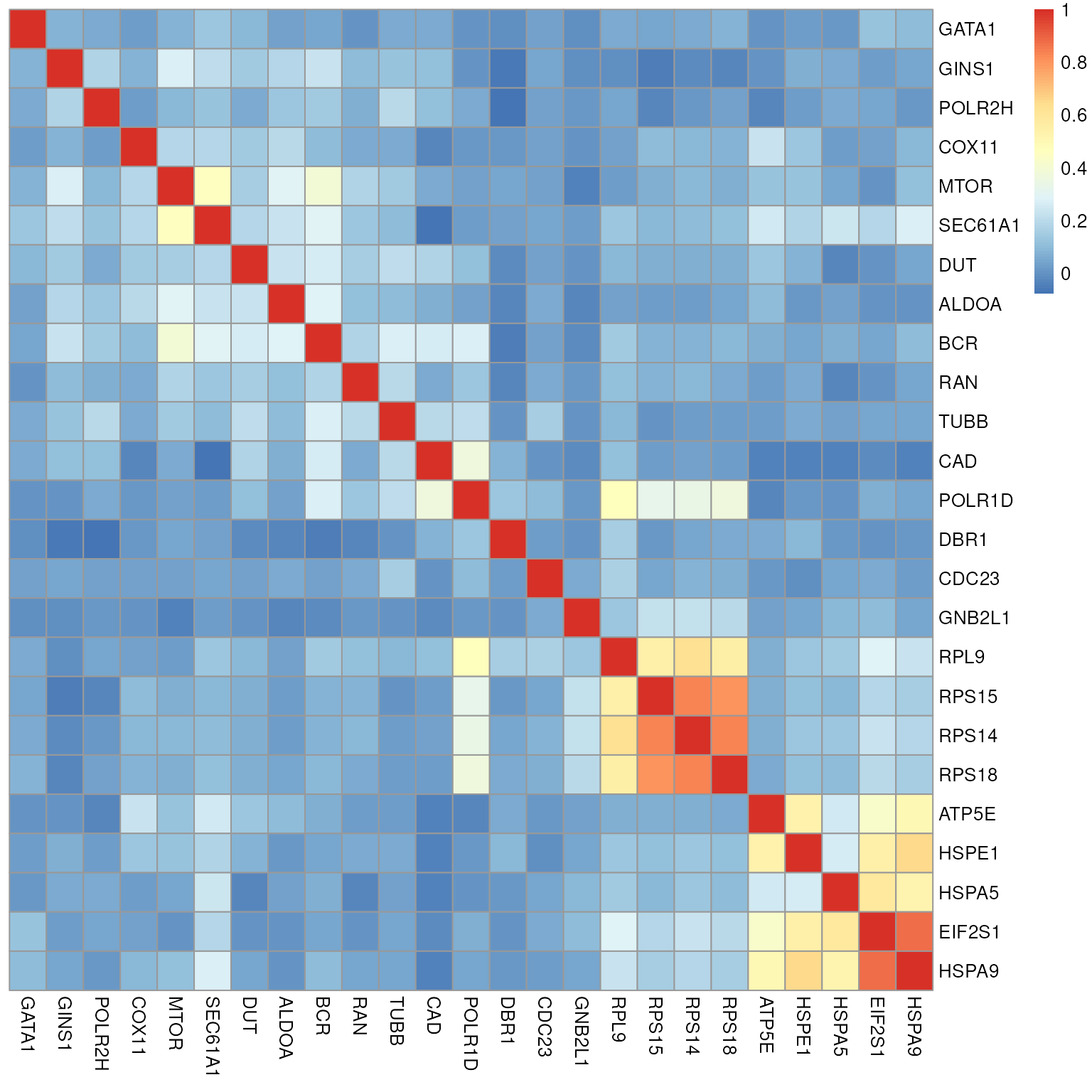
We can visualize relationships among perturbations by looking at the correlation of their fingerprints.
Identifying perturbations in mismatched-guide cells
With a dictionary learned from perfectly matched guides, we can now ask whether the weaker perturbations recover the same fingerprints.
Next, we can map cells from jost_mismatch to this
dictionary of fingerprints. We first demonstrate this at the
group-level, where cells of the same condition can be assigned together.
Here, we map cells according to their perturbation labels, and obtain a
dataframe summarizing these assignments.
jost_mismatch <- FingerprintCells(jost_mismatch, condition_meta = 'gene',
                                  control_class = 'neg', dictionary = dictionary,
                                  group_level = TRUE)
group_level_summary <- SummarizeResults(jost_mismatch, group_level = TRUE,
                                         condition_meta = 'gene', control_class = 'neg')
print(group_level_summary[1:5,])
## top_credible_set.gene top_lbf.gene all_credible_sets.gene all_lbfs.gene
## CAD CAD 4231.79 CAD 4231.79
## SEC61A1 SEC61A1 3074.41 SEC61A1 3074.41
## RPL9 RPL9 3020.07 RPL9 3020.07
## HSPA5 HSPA5 2875.10 HSPA5 2875.1
## DBR1 DBR1 2844.11 DBR1 2844.11
## all_signs.gene
## CAD +
## SEC61A1 +
## RPL9 +
## HSPA5 +
## DBR1 +The columns in this dataframe can be interpreted as follows:
-
top_credible_set: The top identified effect. If there is uncertainty among multiple perturbations, they are separated by commas. If no assignment is made, thenunassignedis returned. -
top_lbf: The log Bayes factor associated with the top credible set. Higher values indicate greater certainty. If no assignment is made, then this is set toNA. -
all_credible_sets: If more than one credible set is found, all credible sets separated by semicolons. -
all_lbfs: All log Bayes factors separated by semicolons. -
all_signs: The signs of the matches made for each perturbation in each credible set. Positive signs indicate a match in the same directionality as the perturbation. Negative signs should generally be interpreted with care.
These values are also added as metadata to the Seurat object, with
each cell containing the information associated with its condition
label. Note that these metadata columns are appended with the condition
metadata suffix by default, if classification is done at the
group-level. A user-specified suffix can also be passed in using the
suffix parameter.
By default, these summaries are ranked by the Bayes factor of the top credible set, with higher Bayes factor assignments indicating greater confidence. Here, we find a high degree of accuracy in the assignments, meaning that the right perturbation is in the top credible set.
Optionally, this summary can also be put into tidy
format, where each individual credible set is described in its own row.
Here, the resulting dataframe is not much different, because only one
credible set happened to be returned for each group.
tidy_summary <- SummarizeResults(jost_mismatch, group_level = TRUE,
                                 condition_meta = 'gene', control_class = 'neg',
                                 tidy = TRUE)
print(tidy_summary[1:10,])
## query cs lbf sign
## 1 CAD CAD 4231.79 +
## 2 SEC61A1 SEC61A1 3074.41 +
## 3 RPL9 RPL9 3020.07 +
## 4 HSPA5 HSPA5 2875.1 +
## 5 DBR1 DBR1 2844.11 +
## 6 EIF2S1 EIF2S1,HSPA9 2520.02 +,+
## 7 POLR2H POLR2H 2144.63 +
## 8 HSPE1 HSPE1 2144.44 +
## 9 DUT DUT 2118.61 +
## 10 POLR1D POLR1D 1951.72 +We can visualize individual assignments for any group using what we
call Long Island City plots, which are inspired by Manhattan plots in
genome-wide association studies. This displays the largest coefficients,
in magnitude, for each perturbation conditional on inclusion in the
model, and sorts the perturbations via hierarchical clustering (default)
or alphabetically. Each identified credible set is indicated with a
different color. Optionally, a faster version can be created by setting
approx = TRUE to show marginal correlations on the y-axis.
Here, we visualize two examples of our matches.
LongIslandCityPlot(jost_mismatch, query = 'CAD', condition_meta = 'gene',
                   control_class = 'neg', dictionary = dictionary,
                   group_level = T, cs = 10)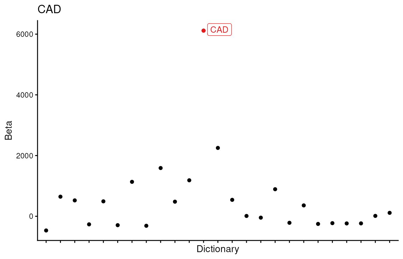
LongIslandCityPlot(jost_mismatch, query = 'EIF2S1', condition_meta = 'gene',
                   control_class = 'neg', dictionary = dictionary,
                   group_level = T, cs = 10)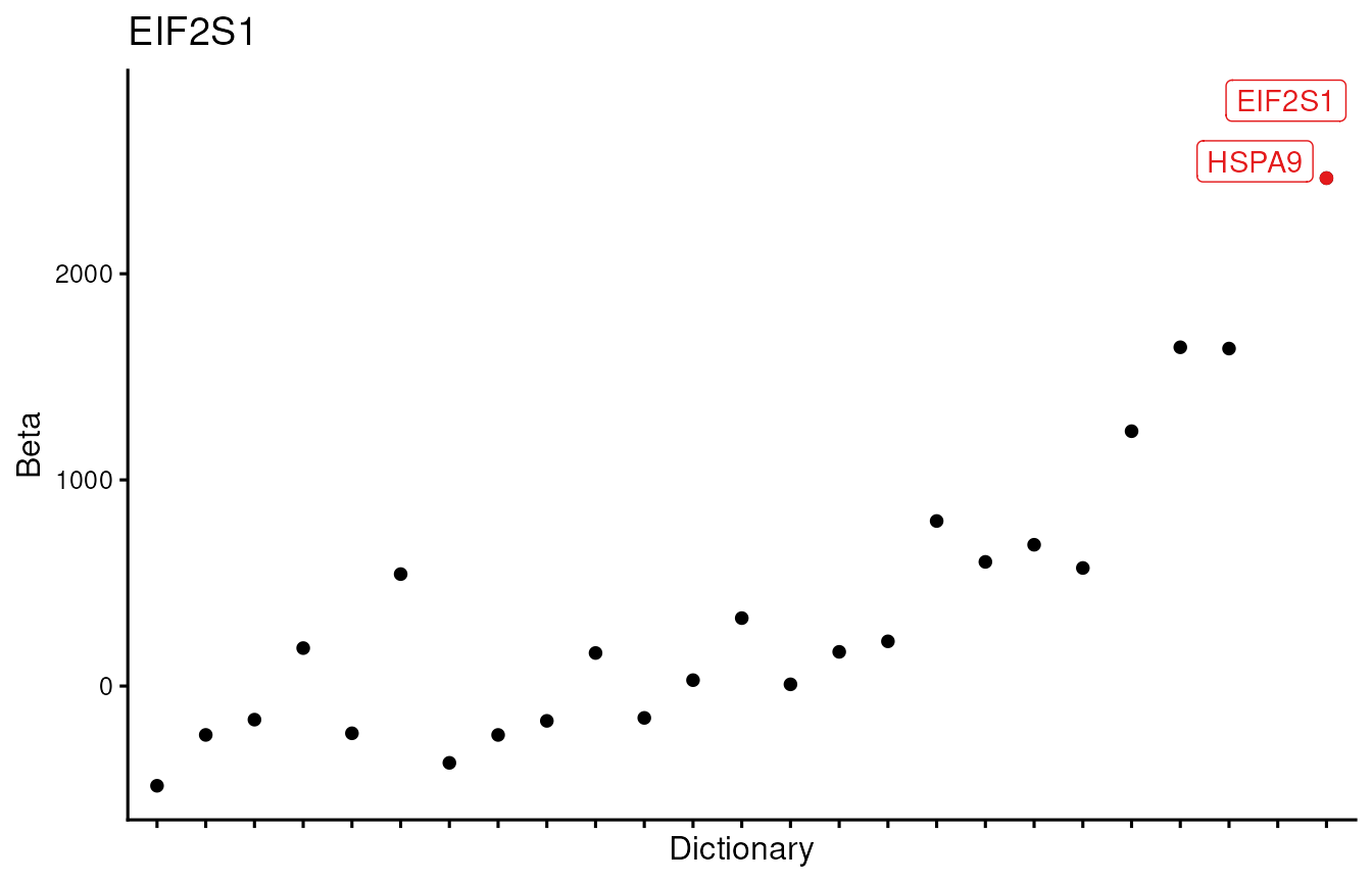
For any given match, we can identify what genes were most responsible
for making that assignment using the ExplainMatch function.
This is done by testing each gene to see which genes, when removed, have
the biggest impact on the Bayes factor. Here, we can identify and print
out the top 25 genes that drove the assignment of CAD-perturbed cells to
CAD by setting plot = FALSE:
ExplainMatch(jost_mismatch, query = 'CAD', match = 'CAD', condition_meta = 'gene',
             control_class = 'neg', dictionary = dictionary,
             group_level = T, num_genes = 25, plot = FALSE)
## genes delta_BF
## AC016629.3 AC016629.3 -85.16326
## MT-CYB MT-CYB -79.26015
## RPLP1 RPLP1 -64.33617
## RPS4X RPS4X -62.87058
## RPS12 RPS12 -62.34242
## MT-CO1 MT-CO1 -60.42173
## BCYRN1 BCYRN1 -57.43327
## PVT1 PVT1 -53.80020
## FTL FTL -51.42681
## UBB UBB -49.37614
## TXNIP TXNIP -49.34610
## APOC1 APOC1 -48.32989
## RPL41 RPL41 -46.09456
## MYL6 MYL6 -43.28774
## UROD UROD -41.94563
## SOD1 SOD1 -41.50352
## RPLP0 RPLP0 -35.72847
## RPL18A RPL18A -35.17677
## MT-CO3 MT-CO3 -33.24842
## DYNLL1 DYNLL1 -33.14542
## SNAPC5 SNAPC5 -30.88845
## GSTP1 GSTP1 -29.62743
## NEAT1 NEAT1 -29.45018
## RPL28 RPL28 -29.34794
## RPL26 RPL26 -27.63253We can also visualize these top genes in both the query data
(jost_mismatch) and the reference data
(jost_match) by using plot = TRUE (which is
the default setting) and specifying details about the reference
object:
ExplainMatch(jost_mismatch, query = 'CAD', match = 'CAD', condition_meta = 'gene',
             control_class = 'neg', dictionary = dictionary,
             group_level = T, ref = jost_match, perturbation_meta = 'gene',
             control_class_ref = 'neg', num_genes = 25)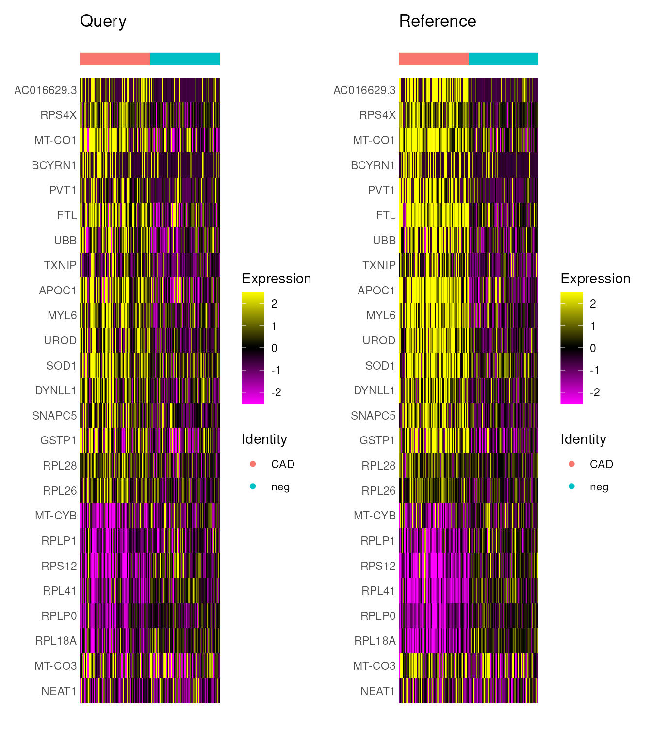
By specifying the include_de parameter, we can
additionally show the top differentially expressed genes in both the
query and the reference data below these top driver genes:
ExplainMatch(jost_mismatch, query = 'CAD', match = 'CAD', condition_meta = 'gene',
             control_class = 'neg', dictionary = dictionary,
             group_level = T, ref = jost_match, perturbation_meta = 'gene',
             control_class_ref = 'neg', num_genes = 25, include_de = 10)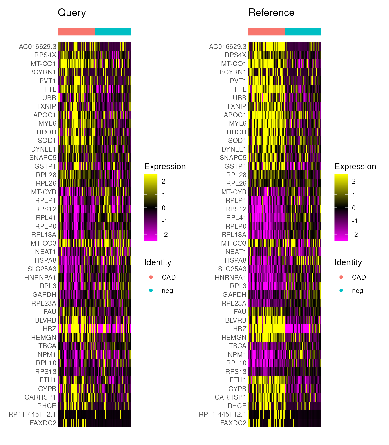
Resolving differences between guides
Pooling cells by target gene can recover a shared response, but it can also hide differences in guide strength.
As an additional example, here we again map cells at the group-level, but this time using their guide identities. Because we want to use all the non-targeting cells as the “control” cells, regardless of the specific non-targeting guide, we create a new metadata column that contains the guide IDs for all the perturbed cells, but just “neg” for each non-targeting cell.
jost_mismatch$guide_identity2 <- jost_mismatch$guide_identity
jost_mismatch$guide_identity2[jost_mismatch$gene == 'neg'] <- 'neg'
Now we can map, specifying the metadata values appropriately:
jost_mismatch <- FingerprintCells(jost_mismatch, condition_meta = 'guide_identity2',
                                  control_class = 'neg', dictionary = dictionary,
                                  group_level = TRUE)
group_level_summary <- SummarizeResults(jost_mismatch, group_level = TRUE,
                                         condition_meta = 'guide_identity2',
                                         control_class = 'neg')
print(group_level_summary[1:5,])
## top_credible_set.guide_identity2
## HSPA5_HSPA5_+_128003624.23-P1P2_08 HSPA5
## HSPA5_HSPA5_+_128003624.23-P1P2_01 HSPA5
## HSPA5_HSPA5_+_128003624.23-P1P2_04 HSPA5
## HSPA5_HSPA5_+_128003624.23-P1P2_06 HSPA5
## CAD_CAD_+_27440280.23-P1P2_03 CAD
## top_lbf.guide_identity2
## HSPA5_HSPA5_+_128003624.23-P1P2_08 11389.10
## HSPA5_HSPA5_+_128003624.23-P1P2_01 10791.31
## HSPA5_HSPA5_+_128003624.23-P1P2_04 10665.02
## HSPA5_HSPA5_+_128003624.23-P1P2_06 4990.00
## CAD_CAD_+_27440280.23-P1P2_03 3981.01
## all_credible_sets.guide_identity2
## HSPA5_HSPA5_+_128003624.23-P1P2_08 HSPA5
## HSPA5_HSPA5_+_128003624.23-P1P2_01 HSPA5
## HSPA5_HSPA5_+_128003624.23-P1P2_04 HSPA5
## HSPA5_HSPA5_+_128003624.23-P1P2_06 HSPA5
## CAD_CAD_+_27440280.23-P1P2_03 CAD
## all_lbfs.guide_identity2
## HSPA5_HSPA5_+_128003624.23-P1P2_08 11389.1
## HSPA5_HSPA5_+_128003624.23-P1P2_01 10791.31
## HSPA5_HSPA5_+_128003624.23-P1P2_04 10665.02
## HSPA5_HSPA5_+_128003624.23-P1P2_06 4990
## CAD_CAD_+_27440280.23-P1P2_03 3981.01
## all_signs.guide_identity2
## HSPA5_HSPA5_+_128003624.23-P1P2_08 +
## HSPA5_HSPA5_+_128003624.23-P1P2_01 +
## HSPA5_HSPA5_+_128003624.23-P1P2_04 +
## HSPA5_HSPA5_+_128003624.23-P1P2_06 +
## CAD_CAD_+_27440280.23-P1P2_03 +In most cases, we still find the expected match for each guide, albeit sometimes with more uncertainty. Among our lowest certainty calls, we do see some mistakes, and occasionally more than one credible set is used. There are also some guides which are left unassigned, indicating that the signal differed enough that we were unable to make a match.
For one of our incorrect assignments, the ExplainMatch
function helps us see that the match is imperfect, which demonstrates
how this visualization can be used to assess whether an assignment makes
sense. While the top driver genes look consistent, the top DE genes from
the reference are not replicated in the query.
ExplainMatch(jost_mismatch, query = 'MTOR_MTOR_+_11322547.23-P1P2_10',
             match = 'GINS1', condition_meta = 'guide_identity2',
             control_class = 'neg', dictionary = dictionary,
             group_level = T, ref = jost_match, perturbation_meta = 'gene',
             control_class_ref = 'neg', num_genes = 25, include_de = 10)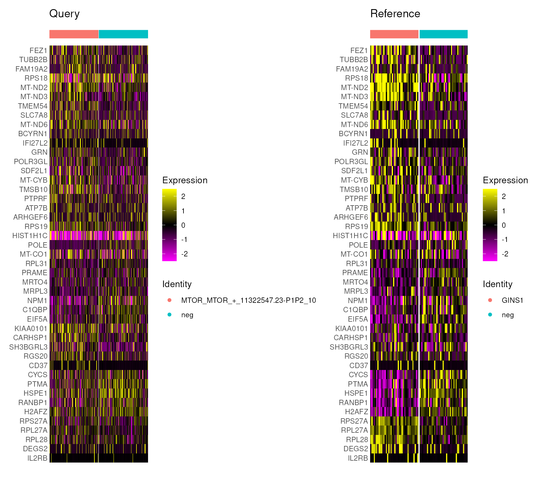
For some of the guides that don’t match, we can look at top DEGs from the reference to understand why:
gata1_degs <- FindMarkers(jost_match, ident.1 = 'GATA1', ident.2 = 'neg',
                          group.by = 'gene')
gata1_degs <- rownames(gata1_degs)[1:25][order(gata1_degs$avg_log2FC[1:25])]
DoHeatmap(jost_mismatch, gata1_degs, group.by = 'guide_identity2', label = F,
          cells = colnames(jost_mismatch)[jost_mismatch$gene %in% c('neg','GATA1')])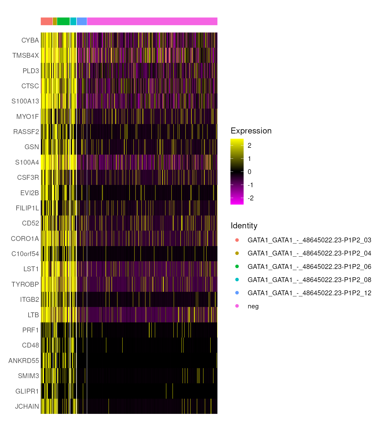
Here, we see that the guide identities in the query that did match indeed show a strong phenotype, whereas the one that didn’t match (GATA1_GATA1_-_48645022.23-P1P2_12) does not show the same gene expression pattern.
Characterizing heterogeneity between individual cells
Having examined differences between guides, we can also ask whether individual cells show the expected response.
We can also map cells on an individual basis by setting
group_level = FALSE. This will be slower than group-level
classification, and we can speed it up by using parallelization with
mc.cores. For example, here, we use 5 cores.
jost_mismatch <- FingerprintCells(jost_mismatch, condition_meta = 'gene',
                                  control_class = 'neg', dictionary = dictionary,
                                  group_level = FALSE, mc.cores = 5)
cell_level_summary <- SummarizeResults(jost_mismatch, group_level = FALSE,
                                       condition_meta = 'gene', control_class = 'neg')
print(head(cell_level_summary))
## gene top_credible_set top_lbf all_credible_sets all_lbfs
## CAGAATCCATTAACCG-2 HSPA5 HSPA5 2951.57 HSPA5 2951.57
## CATTATCTCCGCATAA-2 HSPA5 HSPA5 2857.48 HSPA5 2857.48
## CTCTACGGTCAACATC-2 HSPA5 HSPA5 2795.89 HSPA5 2795.89
## TCAATCTAGCGTCTAT-2 HSPA5 HSPA5 2615.20 HSPA5 2615.2
## CACCTTGGTTACGTCA-2 HSPA5 HSPA5 2561.47 HSPA5 2561.47
## TCAACGATCTCAAGTG-2 HSPA5 HSPA5 2521.62 HSPA5 2521.62
## all_signs
## CAGAATCCATTAACCG-2 +
## CATTATCTCCGCATAA-2 +
## CTCTACGGTCAACATC-2 +
## TCAATCTAGCGTCTAT-2 +
## CACCTTGGTTACGTCA-2 +
## TCAACGATCTCAAGTG-2 +This time, the metadata added to the Seurat object reflects the assignments made for each individual cell. We can confirm that many of these top assignments match the true perturbation labels.
Group-level and cell-level assignments represent a trade-off, where group-level assignments increase power to detect even very subtle signals, but cell-level assignments allow us to better characterize heterogeneity. For example, here we can visualize HSPA5 markers in all the cells that truly received an HSPA5 guide split by their top assigned label.
hspa5_markers <- FindMarkers(jost_match, ident.1 = 'HSPA5', ident.2 = 'neg',
                             group.by = 'gene')
hspa5_markers <- rownames(hspa5_markers)[1:50][order(hspa5_markers$avg_log2FC[1:50])]
DoHeatmap(jost_mismatch, hspa5_markers,
          cells = colnames(jost_mismatch)[jost_mismatch$gene == 'HSPA5'],
          group.by = 'top_credible_set', size = 3, label = F)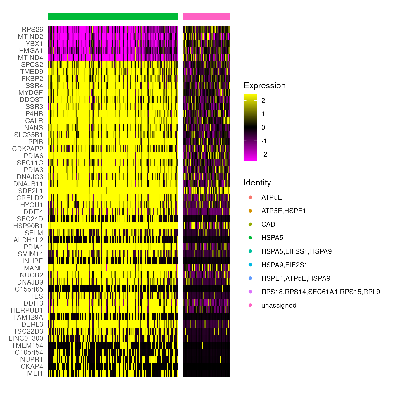
We can see that the majority of these cells either received the specific label HSPA5, or were left unassigned. When comparing these two groups, we see that the cells labeled as HSPA5 strongly show the associated signal, whereas the unassigned cells appear to have escaped the perturbation.
Finally, we can produce a 2D visualization of all assigned cells by
using the ProjectFingerprints function. This projects each
assigned cell onto the fingerprints, which is stored in a
proj assay, and then runs UMAP on those values, which is
stored as the projUMAP reduction. Here, we can label each
cell by its true perturbation:
jost_mismatch <- ProjectFingerprints(jost_mismatch, 'gene', 'neg', dictionary)
DimPlot(jost_mismatch, group.by = 'gene', reduction = 'projUMAP', label = T)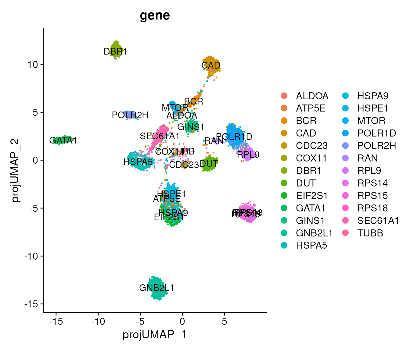
We can see that cells generally separate based on their true perturbation labels, with very similar perturbation classes grouping together.
Mapping to a precomputed GWPS reference
So far, we have learned fingerprints from the same experiment and used them to identify weaker perturbations and differences between cells. We can extend this analysis by using precomputed fingerprints for Genome-Wide Perturb-seq (GWPS). This allows us to compare the query against a larger dictionary without learning fingerprints ourselves.
For this analysis, we return to jost, the filtered
object created at the start of the vignette, which still contains cells
receiving both perfectly matched and mismatched guides. The earlier
normalization and mapping steps operated on jost_match and
jost_mismatch, leaving jost available as the
query for this reference.
First, we normalize the query data with SCTransform;
importantly, we specify return.only.var.genes = FALSE.
jost <- SCTransform(jost, return.only.var.genes = FALSE)Now we can install the precomputed GWPS dictionary from
RNAFingerprintingData. This installation only needs to be
run once. Note that all available dictionaries can be viewed using
AvailableDictionaries().
if (!requireNamespace("gwps", quietly = TRUE)) {
  InstallPrecomputedDictionary(name = 'gwps')
}
Next, we can load in this dictionary using the convenience loader
function LoadPrecomputedDictionary. The GWPS fingerprints
were learned with genes in the ENSEMBL ID format, whereas our query data
uses gene symbols. To make these compatible, we specify
gene_key = 'SYMBOL' when loading it in. More generally, the
ConvertGenes function can be used to update any set of
fingerprints from one gene key type to another.
gwps_dictionary <- LoadPrecomputedDictionary(name = 'gwps', gene_key = 'SYMBOL')As a note, there is likely to be at least some degree of feature mismatch between these GWPS fingerprints and a given query dataset. While this is allowable and unlikely to yield substantive differences in results, this represents an approximation of the procedure and is a trade-off for the convenience of using these pre-computed fingerprints.
Identifying shared responses with GWPS
We can start by trying to map cells from the query data to GWPS at
the group-level, where cells of the same condition can be assigned
together. Here, we map cells according to their perturbation labels, and
obtain a dataframe summarizing these assignments. This can be slow due
to the size of GWPS, but faster results can be obtained using
parallelization with the mc.cores parameter.
jost <- FingerprintCells(jost,
                         condition_meta = 'gene',
                         control_class = 'neg',
                         dictionary = gwps_dictionary,
                         group_level = TRUE)
group_level_summary <- SummarizeResults(jost, group_level = TRUE,
                                         condition_meta = 'gene',
                                         control_class = 'neg')
print(group_level_summary[1:5,])
## top_credible_set.gene
## GATA1 HMBOX1,GATA1
## RPL9 SPATA5L1,URB2,ABCF1,NLE1,CINP,DDX51,RPL3,EIF6,NVL,CENPP,RSL1D1,MYBBP1A,SPATA5,TMA16,HERC1,SURF6,KRR1,UBE2E1,WDR55,NOL9
## RPS14 KRR1,WDR3,FBXL14,RIOK1,AATF,RPS12,DNTTIP2,DDX52,DDX10,WDR36,ZNF84,DIMT1,POP4,RIOK2,DDX47,RPP30,RPS10-NUDT3,ZNHIT6,IMPA2,FCF1,RPS14,RPS3,RPS19,TSR2,AAR2,ZCCHC9,RPS15A,UTP20,RPS3A,RPS20,RPS6,ABT1,RPP14,LAMB1,NAF1,UTP23,RRP12,KRI1
## POLR1D TAF1C,RPL3,TAF1D,GTF3C6,POLR1E,POLR1C,CD3EAP,TAF1A,SPATA5L1,POLR1D
## CAD DHODH,CAD,UQCRFS1,SDHA,UQCRQ,CYCS,IMPDH2,GMPS,UMPS
## top_lbf.gene
## GATA1 2723.73
## RPL9 2676.07
## RPS14 1782.58
## POLR1D 1619.01
## CAD 1610.33
## all_credible_sets.gene
## GATA1 HMBOX1,GATA1
## RPL9 SPATA5L1,URB2,ABCF1,NLE1,CINP,DDX51,RPL3,EIF6,NVL,CENPP,RSL1D1,MYBBP1A,SPATA5,TMA16,HERC1,SURF6,KRR1,UBE2E1,WDR55,NOL9
## RPS14 KRR1,WDR3,FBXL14,RIOK1,AATF,RPS12,DNTTIP2,DDX52,DDX10,WDR36,ZNF84,DIMT1,POP4,RIOK2,DDX47,RPP30,RPS10-NUDT3,ZNHIT6,IMPA2,FCF1,RPS14,RPS3,RPS19,TSR2,AAR2,ZCCHC9,RPS15A,UTP20,RPS3A,RPS20,RPS6,ABT1,RPP14,LAMB1,NAF1,UTP23,RRP12,KRI1
## POLR1D TAF1C,RPL3,TAF1D,GTF3C6,POLR1E,POLR1C,CD3EAP,TAF1A,SPATA5L1,POLR1D
## CAD DHODH,CAD,UQCRFS1,SDHA,UQCRQ,CYCS,IMPDH2,GMPS,UMPS
## all_lbfs.gene
## GATA1 2723.73
## RPL9 2676.07
## RPS14 1782.58
## POLR1D 1619.01
## CAD 1610.33
## all_signs.gene
## GATA1 +,+
## RPL9 +,+,+,+,+,+,+,+,+,+,+,+,+,+,+,+,+,+,+,+
## RPS14 +,+,+,+,+,+,+,+,+,+,+,+,+,+,+,+,+,+,+,+,+,+,+,+,+,+,+,+,+,+,+,+,+,+,+,+,+,+
## POLR1D +,+,+,+,+,+,+,+,+,+
## CAD +,+,+,+,+,+,+,+,+Some of these assignments involve very long credible sets, which
makes sense given that many of these perturbations are of genes
belonging to large complexes. We can visualize these assignments using
Long Island City plots. Below, we show an example of an assignment with
a long credible set, and one with a short credible set. We could
alternatively sort the fingerprints in alphabetical order by setting the
order argument appropriately.
LongIslandCityPlot(jost, query = 'RPS14', condition_meta = 'gene',
                   control_class = 'neg', dictionary = gwps_dictionary,
                   group_level = T, cs = 10)
LongIslandCityPlot(jost, query = 'BCR', condition_meta = 'gene',
                   control_class = 'neg', dictionary = gwps_dictionary,
                   group_level = T, cs = 10)
These plots show the conditional posterior mean coefficients for each
fingerprint on the y-axis. However, in large-scale settings, this can be
slow to compute. For a faster version, we can specify the argument
approx = TRUE to instead show marginal correlations on the
y-axis, e.g.:
LongIslandCityPlot(jost, query = 'RPS14', condition_meta = 'gene',
                   control_class = 'neg', dictionary = gwps_dictionary,
                   group_level = T, cs = 10, approx = TRUE)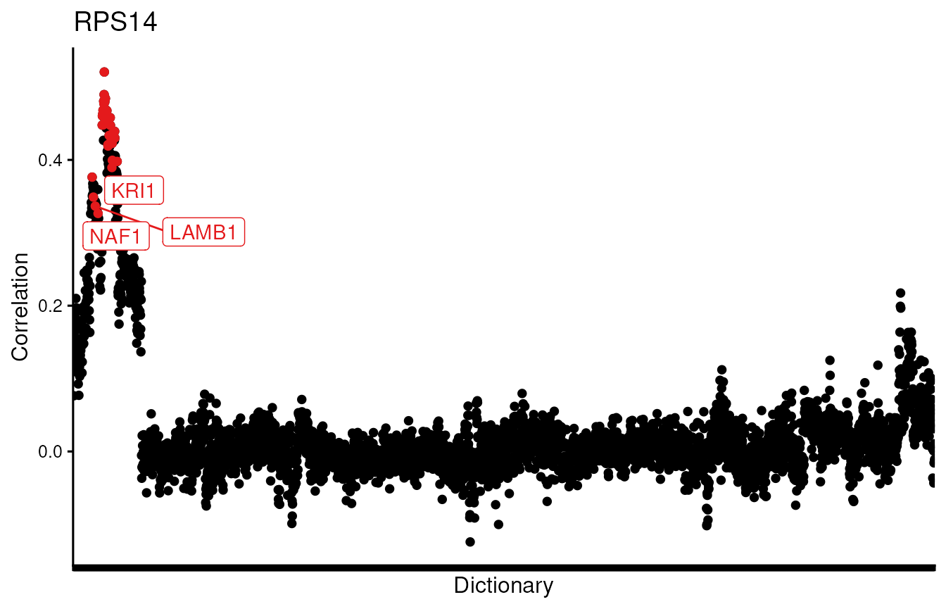
LongIslandCityPlot(jost, query = 'BCR', condition_meta = 'gene',
                   control_class = 'neg', dictionary = gwps_dictionary,
                   group_level = T, cs = 10, approx = TRUE)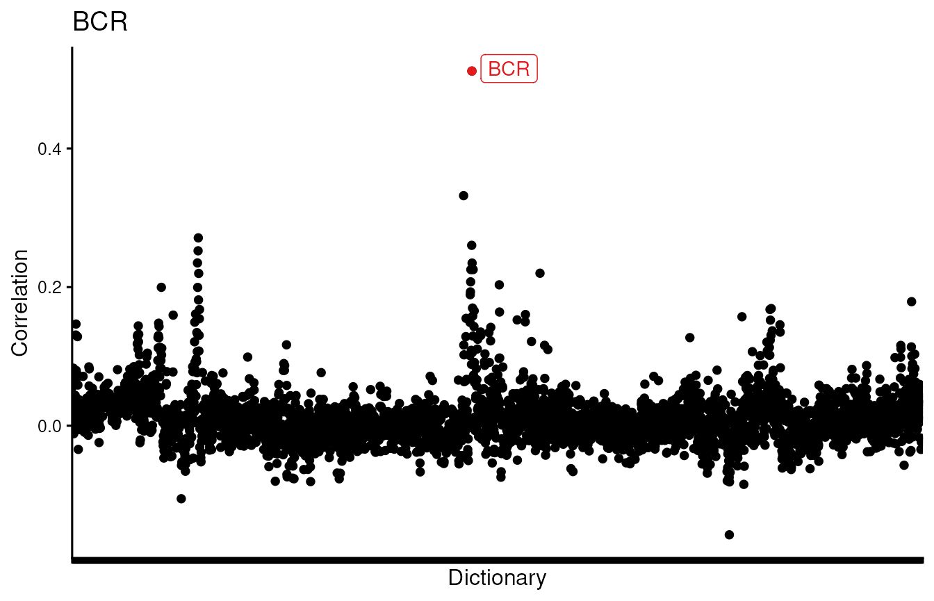
To understand what genes were most responsible for driving these
matches, we can use the ExplainMatch function. Here, the
visualizations are automatically made with the stored pseudobulk GWPS
object inside the precomputed dictionary, since we don’t have the full
GWPS object loaded in.
ExplainMatch(jost, query = 'BCR', match = 'BCR',
             condition_meta = 'gene', control_class = 'neg',
             dictionary = gwps_dictionary, group_level = T,
             num_genes = 25)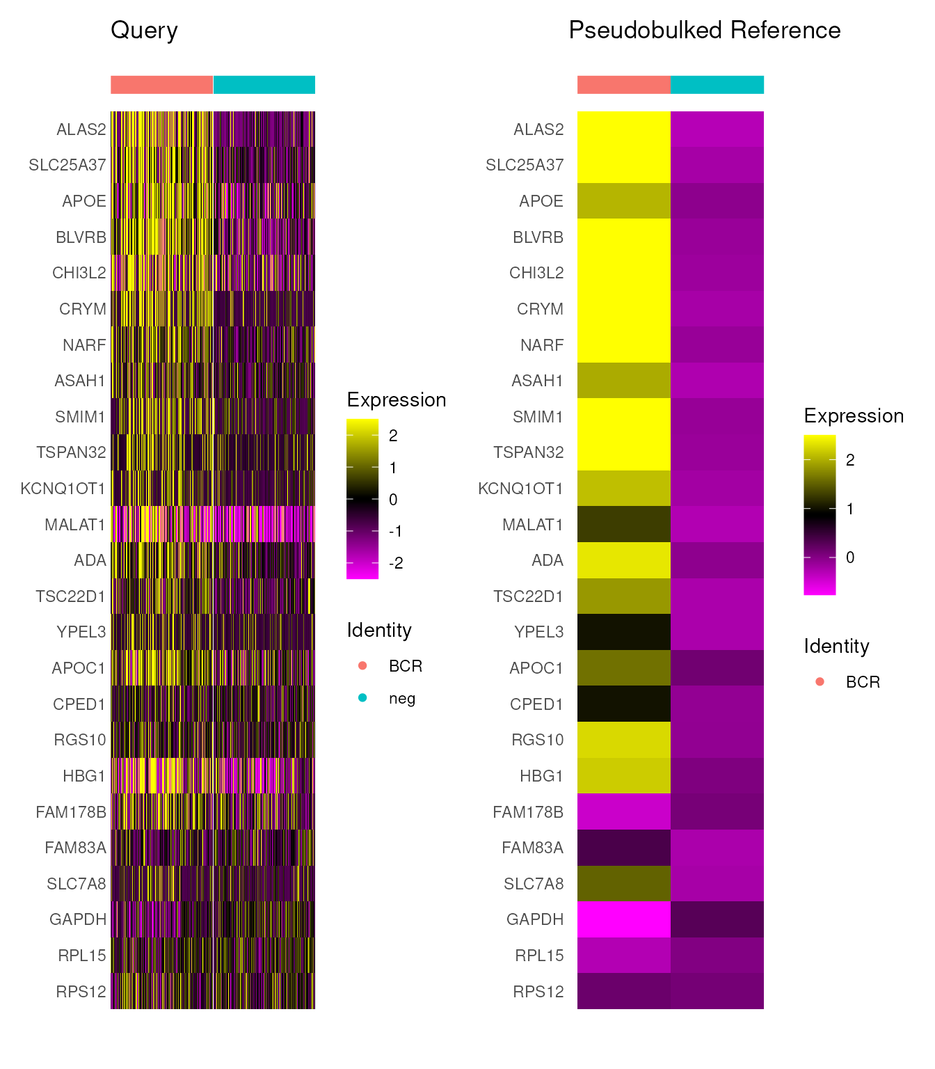
Mapping individual cells to GWPS
We can also map cells on an individual basis. This will be slower
than group-level classification, so here we speed it up by using
parallelization with mc.cores.
jost <- FingerprintCells(jost, condition_meta = 'gene', control_class = 'neg',
                         dictionary = gwps_dictionary,
                         group_level = FALSE, mc.cores = 10)
cell_level_summary <- SummarizeResults(jost, group_level = FALSE,
                                       condition_meta = 'gene',
                                       control_class = 'neg')
print(head(cell_level_summary))
## gene
## CAGTAACAGAGGGCTT-2 RPL9
## GCAGTTACAAGCTGGA-2 RPL9
## ATCACGACAGGTCGTC-2 RPL9
## TTGGAACTCATGGTCA-1 RPL9
## TTCCCAGCACGCTTTC-2 RPL9
## TGCGGGTAGTGGACGT-2 RPL9
## top_credible_set
## CAGTAACAGAGGGCTT-2 ABCF1,CINP,DDX24,NLE1,URB2,SPATA5L1,EIF6,KIF18B,RPL8,RPL5,RPL36,RPL30,RPL24,SDAD1,MYBBP1A,GNL2,PES1,WDR12,RPS7,TSR2,EIF3A,RPS4X,RPS3,RPS6,KRR1,RPS9,DDX47,UTP20,TTF1,CENPP,FBL,SOX3,NIFK,RPL18,GLIS1,RPS15A,STK24,DDX51,RPL34
## GCAGTTACAAGCTGGA-2 RPL24,RPL10,RPL19,RPL30,ABCF1,NLE1,URB2,DDX51,TEX10,RSL1D1,CINP,SPATA5L1,GLIS1,EIF6,RPL10A
## ATCACGACAGGTCGTC-2 RPL5,RPL10,RPL30,RPL24,RPL38,RPL37,RPLP0,RPL13,SDAD1,NLE1,EIF6,URB2,MAK16,DDX51,DDX56,ABCF1,NOP16,DDX24,RPL11,EBNA1BP2,GLIS1,RPL31,RPL36,RRS1,SPATA5L1,CINP,CENPP,DNTTIP2,CARF,HDAC6,WDR12,SURF6,TEX10,RSL24D1
## TTGGAACTCATGGTCA-1 ABCF1,NLE1,SDAD1,GNL2,RPL36,DDX24,URB2,DDX55,RRS1,CINP,MAK16,SPATA5L1,NOC3L,RPS20,AATF,RPS3,RPS6,RPS24,RPS12,DDX47,RPL13,RPL7,RPL34,RPL37A,RPL18,RPL8,RPL4,RPL24,RPL17,RPLP0,GLIS1,CENPP,WDR12,CARF
## TTCCCAGCACGCTTTC-2 URB2,NVL,MYBBP1A,RSL1D1,TMA16,SPATA5L1,BOP1,TEX10,ZNHIT6,KRR1,DIMT1,TSR2,DDX52,DDX18,RPS19,FBL,ABCF1,CINP,CARF,GNL2,MAK16,KIF18B,SURF6,DDX54,CEBPZ,RPS20,FERMT2,EIF6,DDX51,PPAN,NIFK,GTPBP4,RCL1,RPS6,SDAD1,DDX55,NSA2,HDAC6,LAS1L,CENPP,RRS1,SUMO1,NOL8,GLIS1,DDX47,RPS3,PES1,RPS9,NLE1,RPS12,NOP2,NMD3,DNTTIP2,RRP12,LTV1
## TGCGGGTAGTGGACGT-2 ABCF1,URB2,EIF6,SPATA5L1,TEX10,NLE1,DDX56,NIFK,DDX55,SDAD1,DDX24,GNL2,RRS1,RPL18,RPL21,CENPP,NOC3L,DDX51,CARF,SYNCRIP,TTF1,KRR1,SPATA5,RPL36,NMD3,RPL10,RPLP0,SOX3,MAK16,RPL9,RPL34,KIF18B,HDAC6,RPL31,FERMT2,RPL24,RPL11,LSG1,RPL13A,NIP7,RPL8,NSA2,UBE2E1,NOL8,RPL5,TSR2,EBNA1BP2,SURF6,RSL24D1,FBL,GLIS1,CINP
## top_lbf
## CAGTAACAGAGGGCTT-2 784.83
## GCAGTTACAAGCTGGA-2 753.21
## ATCACGACAGGTCGTC-2 479.00
## TTGGAACTCATGGTCA-1 476.31
## TTCCCAGCACGCTTTC-2 475.13
## TGCGGGTAGTGGACGT-2 473.88
## all_credible_sets
## CAGTAACAGAGGGCTT-2 ABCF1,CINP,DDX24,NLE1,URB2,SPATA5L1,EIF6,KIF18B,RPL8,RPL5,RPL36,RPL30,RPL24,SDAD1,MYBBP1A,GNL2,PES1,WDR12,RPS7,TSR2,EIF3A,RPS4X,RPS3,RPS6,KRR1,RPS9,DDX47,UTP20,TTF1,CENPP,FBL,SOX3,NIFK,RPL18,GLIS1,RPS15A,STK24,DDX51,RPL34
## GCAGTTACAAGCTGGA-2 RPL24,RPL10,RPL19,RPL30,ABCF1,NLE1,URB2,DDX51,TEX10,RSL1D1,CINP,SPATA5L1,GLIS1,EIF6,RPL10A
## ATCACGACAGGTCGTC-2 RPL5,RPL10,RPL30,RPL24,RPL38,RPL37,RPLP0,RPL13,SDAD1,NLE1,EIF6,URB2,MAK16,DDX51,DDX56,ABCF1,NOP16,DDX24,RPL11,EBNA1BP2,GLIS1,RPL31,RPL36,RRS1,SPATA5L1,CINP,CENPP,DNTTIP2,CARF,HDAC6,WDR12,SURF6,TEX10,RSL24D1
## TTGGAACTCATGGTCA-1 ABCF1,NLE1,SDAD1,GNL2,RPL36,DDX24,URB2,DDX55,RRS1,CINP,MAK16,SPATA5L1,NOC3L,RPS20,AATF,RPS3,RPS6,RPS24,RPS12,DDX47,RPL13,RPL7,RPL34,RPL37A,RPL18,RPL8,RPL4,RPL24,RPL17,RPLP0,GLIS1,CENPP,WDR12,CARF
## TTCCCAGCACGCTTTC-2 URB2,NVL,MYBBP1A,RSL1D1,TMA16,SPATA5L1,BOP1,TEX10,ZNHIT6,KRR1,DIMT1,TSR2,DDX52,DDX18,RPS19,FBL,ABCF1,CINP,CARF,GNL2,MAK16,KIF18B,SURF6,DDX54,CEBPZ,RPS20,FERMT2,EIF6,DDX51,PPAN,NIFK,GTPBP4,RCL1,RPS6,SDAD1,DDX55,NSA2,HDAC6,LAS1L,CENPP,RRS1,SUMO1,NOL8,GLIS1,DDX47,RPS3,PES1,RPS9,NLE1,RPS12,NOP2,NMD3,DNTTIP2,RRP12,LTV1
## TGCGGGTAGTGGACGT-2 ABCF1,URB2,EIF6,SPATA5L1,TEX10,NLE1,DDX56,NIFK,DDX55,SDAD1,DDX24,GNL2,RRS1,RPL18,RPL21,CENPP,NOC3L,DDX51,CARF,SYNCRIP,TTF1,KRR1,SPATA5,RPL36,NMD3,RPL10,RPLP0,SOX3,MAK16,RPL9,RPL34,KIF18B,HDAC6,RPL31,FERMT2,RPL24,RPL11,LSG1,RPL13A,NIP7,RPL8,NSA2,UBE2E1,NOL8,RPL5,TSR2,EBNA1BP2,SURF6,RSL24D1,FBL,GLIS1,CINP
## all_lbfs
## CAGTAACAGAGGGCTT-2 784.83
## GCAGTTACAAGCTGGA-2 753.21
## ATCACGACAGGTCGTC-2 479
## TTGGAACTCATGGTCA-1 476.31
## TTCCCAGCACGCTTTC-2 475.13
## TGCGGGTAGTGGACGT-2 473.88
## all_signs
## CAGTAACAGAGGGCTT-2 +,+,+,+,+,+,+,+,+,+,+,+,+,+,+,+,+,+,+,+,+,+,+,+,+,+,+,+,+,+,+,+,+,+,+,+,+,+,+
## GCAGTTACAAGCTGGA-2 +,+,+,+,+,+,+,+,+,+,+,+,+,+,+
## ATCACGACAGGTCGTC-2 +,+,+,+,+,+,+,+,+,+,+,+,+,+,+,+,+,+,+,+,+,+,+,+,+,+,+,+,+,+,+,+,+,+
## TTGGAACTCATGGTCA-1 +,+,+,+,+,+,+,+,+,+,+,+,+,+,+,+,+,+,+,+,+,+,+,+,+,+,+,+,+,+,+,+,+,+
## TTCCCAGCACGCTTTC-2 +,+,+,+,+,+,+,+,+,+,+,+,+,+,+,+,+,+,+,+,+,+,+,+,+,+,+,+,+,+,+,+,+,+,+,+,+,+,+,+,+,+,+,+,+,+,+,+,+,+,+,+,+,+,+
## TGCGGGTAGTGGACGT-2 +,+,+,+,+,+,+,+,+,+,+,+,+,+,+,+,+,+,+,+,+,+,+,+,+,+,+,+,+,+,+,+,+,+,+,+,+,+,+,+,+,+,+,+,+,+,+,+,+,+,+,+We can visualize these assignments by using the
ProjectFingerprints function to create a UMAP of the
projections of each assigned cell onto the fingerprints. Below, we
overlay the plot with each cell’s true perturbation label:
jost <- ProjectFingerprints(jost, 'gene',
                            'neg', gwps_dictionary)
DimPlot(jost, group.by = 'gene',
        reduction = 'projUMAP', label = T)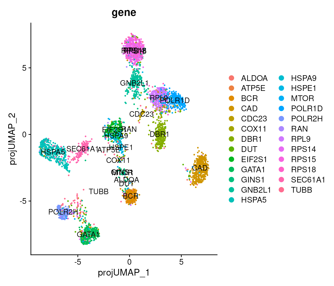
The custom dictionary lets us test how well fingerprints transfer from perfectly matched to mismatched guides, while the precomputed GWPS dictionary places these responses in a larger perturbation reference. In both analyses, group-level assignments help detect shared signals, and individual-cell assignments reveal heterogeneity within a perturbation.
Session Info
sessioninfo::session_info(pkgs = "attached")## ─ Session info ───────────────────────────────────────────────────────────────
## setting value
## version R version 4.5.2 (2025-10-31)
## os Ubuntu 24.04.4 LTS
## system x86_64, linux-gnu
## ui X11
## language en
## collate en_US.UTF-8
## ctype en_US.UTF-8
## tz Etc/UTC
## date 2026-11-06
## pandoc 3.9 @ /usr/bin/ (via rmarkdown)
## quarto 1.8.25 @ /usr/local/bin/quarto
##
## ─ Packages ───────────────────────────────────────────────────────────────────
## package * version date (UTC) lib source
## future * 1.76.0 2026-09-24 [3] CRAN (R 4.5.2)
## pheatmap * 1.0.13 2025-06-05 [3] CRAN (R 4.5.2)
## RNAFingerprinting * 0.0.0.9000 2026-11-06 [3] local
## RNAFingerprintingData * 0.1.0 2026-11-06 [3] local
## Seurat * 6.0.0 2026-11-06 [1] local
## SeuratObject * 5.4.0 2026-04-11 [3] RSPM (R 4.5.0)
## sp * 2.2-4 2026-10-11 [3] RSPM (R 4.5.0)
## stringr * 1.6.0 2025-11-04 [3] RSPM (R 4.5.0)
##
## [1] /scratch/build-QLRyQPI9/library
## [2] /usr/local/lib/R/custom-lib
## [3] /usr/local/lib/R/site-library
## [4] /usr/local/lib/R/library
## * ── Packages attached to the search path.
##
## ──────────────────────────────────────────────────────────────────────────────