Loading and visualizing 10x Atera data
Compiled: November 06, 2026
Source:vignettes/atera_tutorial.Rmd
atera_tutorial.RmdOverview
Note: This tutorial demonstrates how to use Seurat with 10x Atera data. A full vignette will be published at a later date.
In this tutorial, we analyze an Atera FFPE human kidney dataset with Seurat. We load cell-level counts and spatial coordinates, visualize individual transcripts and codewords, and examine cell boundaries in a selected region. We then use a sketch of the dataset to identify clusters and project the results back to all cells.
We use the publicly available Atera In Situ Gene Expression, FFPE Human Kidney dataset from 10x Genomics. This non-diseased tissue sample was profiled with the Atera Human Whole Transcriptome Assay (WTA) and processed with Atera Onboard Analysis v1.0.4.
The workflow keeps the full count matrix on disk with BPCells and performs clustering on a smaller sketch of cells. Transcript coordinates are fetched for selected genes, while cell boundaries are loaded only for a cropped region. These choices reduce the memory needed to explore the tissue.
Load libraries
We load the analysis and plotting libraries below and configure
parallel processing. Setting a future plan controls the
number of processes used for Atera reads. setThreads()
controls threading in downstream Seurat functions independently.
The blosc package is required for reading compressed
Zarr arrays.
if (!requireNamespace("blosc", quietly = TRUE)) {
  install.packages("blosc")
}Load the Atera dataset
We use LoadAtera() to create a Seurat object containing
the counts, cell centroids, and a handle for fetching transcript
coordinates.
Download
and extract the Atera FFPE human kidney dataset from 10x Genomics,
and set data_dir to the extracted directory. The bundle
contains expression matrices, cell boundaries, transcript coordinates,
and morphology images.
To keep the analysis practical for large datasets, we store counts on
disk with BPCells by specifying a cache directory with
bpcells_dir. We recommend using a separate cache for each
dataset, and reusing that cache for subsequent analyses. Opening an
existing cache avoids rebuilding the count matrices, but transcript
coordinates are still read separately when requested. Here, we defer
segmentations until we select a region of interest and skip morphology
images.
data_dir <- "/brahms/zhangbr/vignette_data/atera_kidney"
bpcells_dir <- "atera-kidney-bpcells"
atera_obj <- LoadAtera(data.dir = data_dir,
                      fov = "fov",
                      assay = "Atera",
                      cell.centroids = TRUE,
                      molecule.coordinates = TRUE,
                      bpcells.dir = bpcells_dir,
                      segmentations = NULL,
                      cell.annotations = TRUE,
                      morphology.image = FALSE)

atera_obj
## An object of class Seurat
## 24674 features across 399120 samples within 6 assays
## Active assay: Atera (18049 features, 0 variable features)
## 1 layer present: counts
## 5 other assays present: DeprecatedCodeword, BlankCodeword, ControlCodeword, ControlProbe, GenomicControl
## 1 spatial field of view present: fovIn this dataset, Atera is the gene-expression assay used
for normalization and clustering. The other assays store the non-gene
feature categories, with the spatial and morphological information
required for downstream visualization and analysis.
Assays(atera_obj)## [1] "Atera" "DeprecatedCodeword" "BlankCodeword"
## [4] "ControlCodeword" "ControlProbe" "GenomicControl"Cell type annotations
The Atera Onboard Analysis pipeline performs cell type annotation with Pan-human Azimuth for human samples by default.
LoadAtera() will add the azimuth_* columns
from obs in cell_feature_matrix.zarr.zip to
the Seurat object metadata by default if they are available, or if
specified via the cell.annotations parameter as we did
above.
Annotations by themselves can also be requested with
ReadAtera(); for example:
annotations <- ReadAtera(data.dir = data_dir, outs = "annotations")$annotations.
annotation.columns <- grep("^azimuth_", colnames(atera_obj[[]]), value = TRUE)

tail(atera_obj[[]][, annotation.columns])
## azimuth_broad azimuth_coarse
## 8199291971 Endothelial cell Endothelial cell
## 8199292807 Immune cell B cell
## 8199308871 Perivascular cell Vascular smooth muscle cell
## 8199311332 Unassigned Unassigned
## 8199332461 Unassigned Unassigned
## 8199348186 Unassigned Unassigned
## azimuth_fine azimuth_score
## 8199291971 Capillary EC 0.6097147
## 8199292807 Plasma cell 0.4555703
## 8199308871 Vascular smooth muscle cell 0.9319242
## 8199311332 Unassigned 0.9868732
## 8199332461 Unassigned 0.9960636
## 8199348186 Unassigned 0.8666266
## azimuth_full_hierarchy
## 8199291971 Endothelial cell|Capillary EC
## 8199292807 Immune cell|Lymphoid cell|B cell|Plasma cell
## 8199308871 Perivascular cell|Vascular smooth muscle cell
## 8199311332 Unassigned
## 8199332461 Unassigned
## 8199348186 UnassignedBelow, we see how (broad) cell types are organized within the kidney tissue:
ImageDimPlot(atera_obj,
            fov = "fov",
            group.by = "azimuth_broad",
            size = 0.1) + ggtitle("azimuth_broad")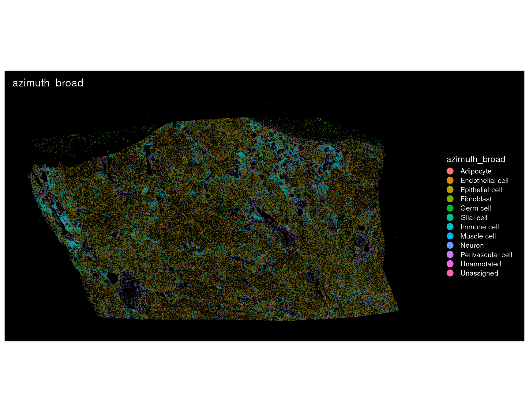
Visualize spatial data
ImageDimPlot() and ImageFeaturePlot()
display Atera coordinates with x horizontally and y increasing downward,
matching the morphology images’ top-left origin. Stored coordinates
remain unchanged. We use these same tissue coordinates when cropping the
field of view below. To reproduce the older plot layout, set
flip_xy = TRUE in either plotting function.
Quality control
We first visualize the number of transcripts and genes detected per cell. Spatial variation in these values can help identify regions worth inspecting more closely, but differences can also reflect cell size and tissue composition. We therefore examine these maps alongside the cell boundaries rather than choosing a single cutoff from the plots alone.
p1 <- ImageFeaturePlot(atera_obj,
                      fov = "fov",
                      features = "nCount_Atera",
                      size = 1) + ggtitle("Transcript counts per cell")

p2 <- ImageFeaturePlot(atera_obj,
                      fov = "fov",
                      features = "nFeature_Atera",
                      size = 1) + ggtitle("Genes detected per cell")

p1 + p2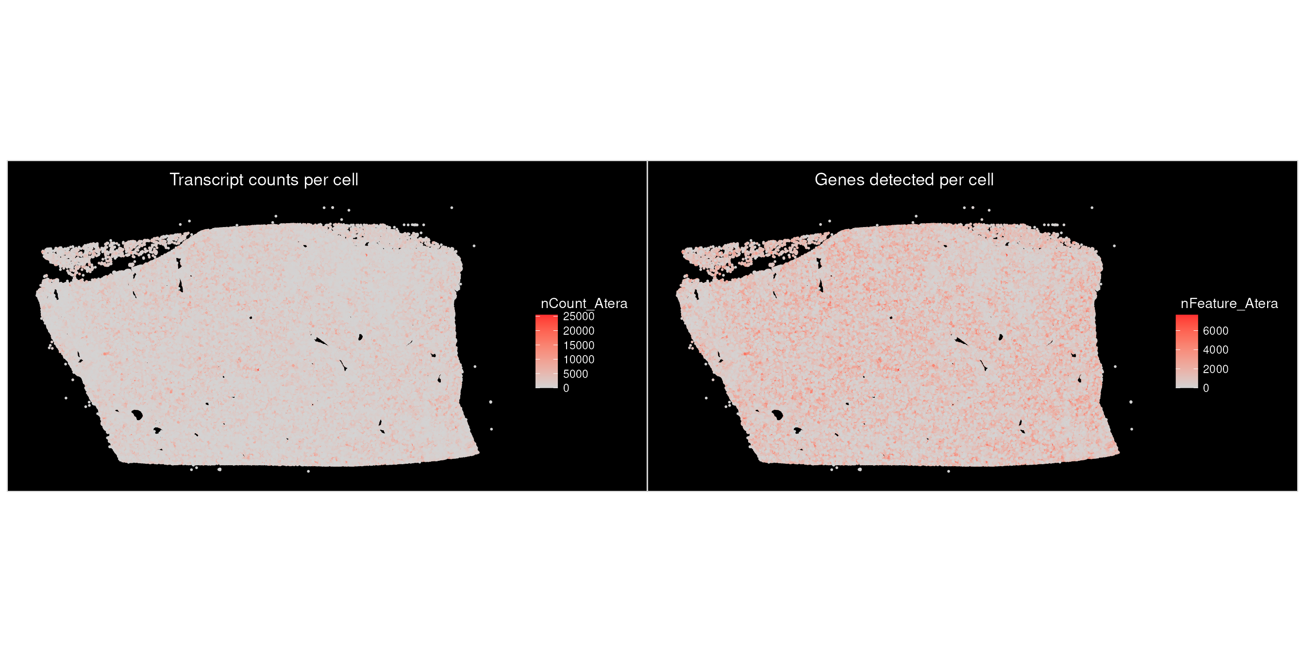
Visualize individual transcripts
Transcript coordinates are fetched on demand with
LoadAteraMolecules(). Here, we retrieve coordinates for
PDK1. Subsequent calls reuse coordinates that have already been
loaded.
The transcript file stores physical coordinates and calibrated
quality scores for individual detections. The file contains all decoded
transcripts, whereas the cell-feature matrix uses transcripts that pass
the default quality value (Q-Score) threshold of Q20.
LoadAtera() defaults to mols.qv.threshold = 20
for gene-level molecule reads.
gene_name <- "PDK1"

atera_obj <- LoadAteraMolecules(atera_obj, genes = gene_name)
We overlay the molecules on cell centroids, using orange to distinguish transcripts from the gray tissue background.
p3 <- ImageDimPlot(atera_obj,
                  fov = "fov",
                  # Only centroids have been loaded; segmentation polygons are not yet available.
                  boundaries = NULL,
                  size = 0.1,
                  cols = "grey80",
                  molecules = gene_name,
                  mols.size = 0.1,
                  mols.cols = "orange",
                  axes = TRUE) + ggplot2::ggtitle(paste(gene_name, "transcripts"))

p3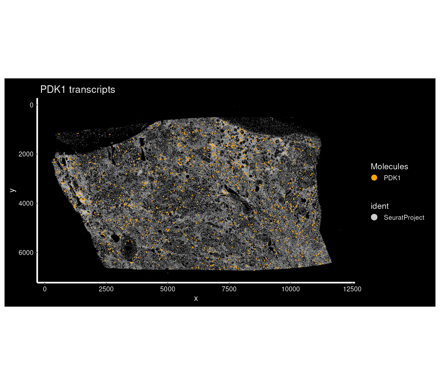
We can also compare the spatial distributions of multiple genes of interest. Let’s look at COL4A5 in addition to PDK1, first loading the molecules for both genes.
genes <- c("PDK1", "COL4A5")

atera_obj <- LoadAteraMolecules(atera_obj, genes = genes)
Next, we can visualize both genes together on the same plot of the
tissue. The colors identify which gene each displayed molecule belongs
to, so these visualizations help us inspect whether signals occupy
similar tissue regions or different cellular neighborhoods. It may be
helpful to adjust mols.size for the field of view, as
larger sizes can obscure spatial detail in dense regions.
p4 <- ImageDimPlot(atera_obj,
                    fov = "fov",
                    boundaries = NULL,
                    size = 0.1,
                    cols = "grey80",
                    molecules = genes,
                    mols.size = 0.1,
                    mols.cols = c("orange", "cyan"),
                    axes = TRUE) + ggtitle("Multi-gene transcripts")
p4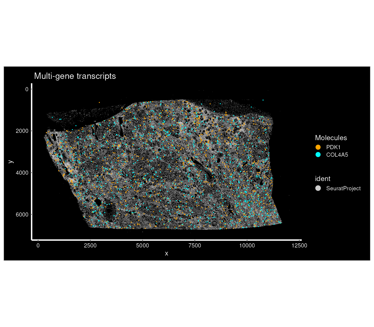
Compare codewords for a gene
A gene can be represented by multiple codewords.
LoadAteraCodewords() retrieves their identities and stores
their coordinates under labels such as
COL4A5_codeword_<id>. We can compare the codewords
together or plot them separately.
The transcript archive records a codeword_identity for
each detection and a mapping from codewords to genes. Comparing the
individual panels can reveal whether codewords show similar spatial
distributions.
This reader retrieves codeword detections (without applying the gene-level molecule quality filter that we used for the gene-level plots).
gene_name <- "COL4A5"
atera_obj <- LoadAteraCodewords(atera_obj, data.dir = data_dir, genes = gene_name)
codeword.labels <- sort(unique(grep(paste0("^", gene_name, "_codeword_"),
                        Misc(atera_obj, "atera.molecules")$cache$gene, value = TRUE)))

cat(length(codeword.labels), "codewords for", gene_name, "\n")
## 3 codewords for COL4A5
# Extend the palette if a gene has more codewords.
palette <- c("orange", "cyan", "magenta", "yellow", "green", "red")

p5 <- ImageDimPlot(atera_obj,
                  fov = "fov",
                  boundaries = NULL,
                  size = 0.1,
                  cols = "grey80",
                  molecules = codeword.labels,
                  mols.size = 0.1,
                  mols.cols = palette[seq_along(codeword.labels)],
                  axes = TRUE) + ggtitle(paste(gene_name, "transcripts by codeword"))
p5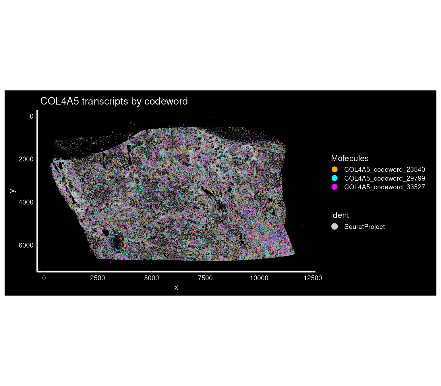
plots <- lapply(codeword.labels, function(cw) {
                ImageDimPlot(atera_obj,
                            fov = "fov",
                            boundaries = NULL,
                            size = 0.1,
                            cols = "grey80",
                            molecules = cw,
                            mols.size = 0.1,
                            mols.cols = "orange",
                            axes = TRUE) + ggtitle(cw) })

p6 <- wrap_plots(plots, ncol = length(plots))
p6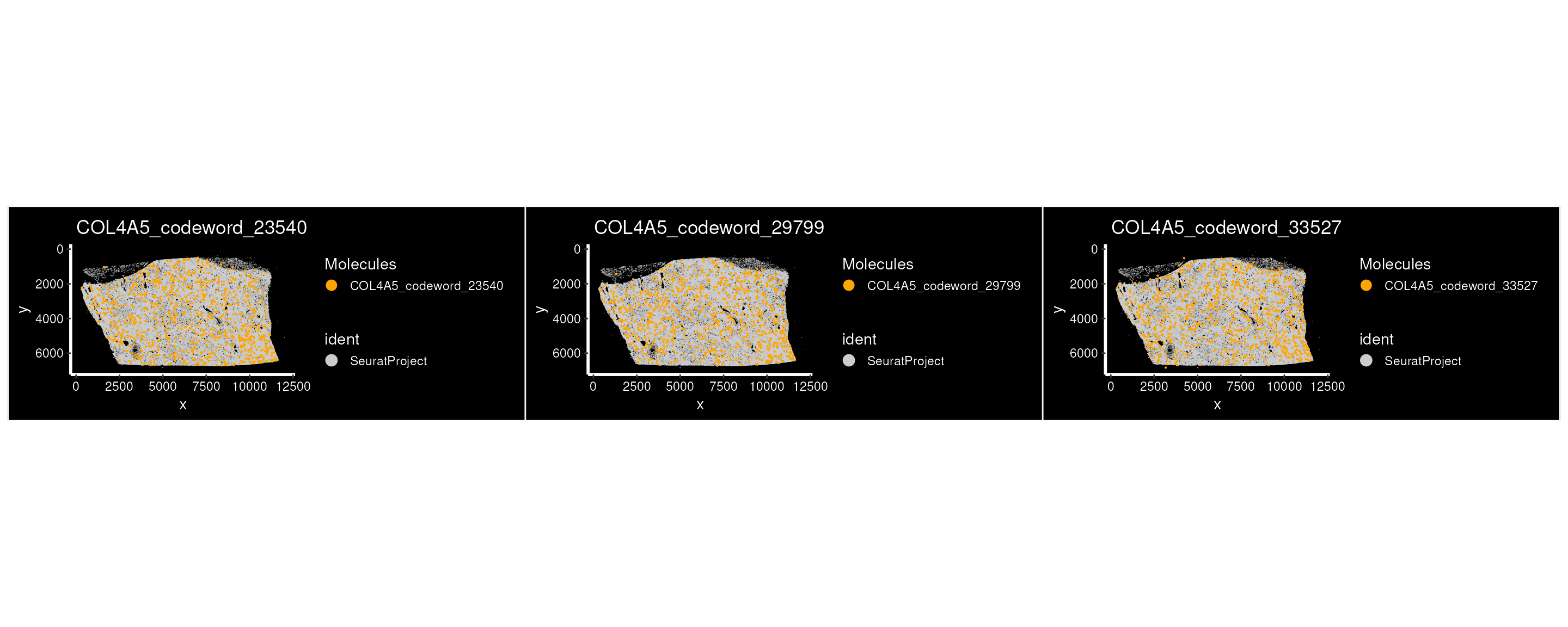
Explore a region of interest
Crop the tissue and load cell boundaries
Cell boundaries and individual molecules are easier to inspect in a
smaller field of view. We can use Crop() to define a region
in tissue coordinates, then load segmentation boundaries for the cells
in that crop.
Creating fov.crop preserves the original field of view
so that we can return to whole-tissue plots at a later stage. The crop
ranges below are in microns based on the tissue coordinate system.
Setting coords = "tissue" makes Crop() use the
original x/y ranges directly.
Loading polygons only for this crop avoids constructing boundaries
for every cell in the bundle. Change crop.x and
crop.y when working with another sample; these coordinates
select a region of the kidney dataset used here.
crop.x <- c(5000, 5200)
crop.y <- c(2000, 2200)

atera_obj[["fov.crop"]] <- Crop(atera_obj[["fov"]],
                                x = crop.x,
                                y = crop.y,
                                coords = "tissue")

atera_obj <- LoadAteraSegmentations(atera_obj,
                                    data.dir = data_dir,
                                    fov = "fov.crop",
                                    segmentations = "cell")

atera_obj <- LoadAteraMolecules(atera_obj, genes = "COL4A5")
We can now visualize transcripts relative to the cell boundaries in this region. The white polygons show cell outlines, while orange points show the selected gene. Looking at their relative positions provides a closer view of the signal than a cell-level expression map alone.
p7 <- ImageDimPlot(atera_obj,
                  fov = "fov.crop",
                  boundaries = "segmentations",
                  cols = "white",
                  axes = TRUE,
                  molecules = "COL4A5",
                  mols.size = 1,
                  mols.cols = "orange",
                  coord.fixed = TRUE)
p7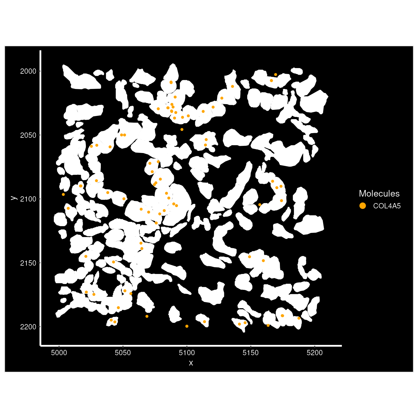
Preprocessing and unsupervised analysis
Analyze a sketch of the dataset
Rather than running dimensional reduction and clustering on every
cell, we select a sketch of 50,000 cells with SketchData().
We normalize the full assay and identify variable features before
sampling the sketch.
The LeverageScore method favors cells that contribute
distinct expression patterns, helping retain variation that uniform
subsampling can miss. The sketch becomes a separate in-memory assay,
while the full count matrix remains available in the BPCells-backed
Atera assay. The sketch size can be adjusted to the dataset
and available memory.
set.seed(42)
setThreads(8) # set the number of threads for parallel processing

DefaultAssay(atera_obj) <- "Atera"
atera_obj <- NormalizeData(atera_obj)

atera_obj <- FindVariableFeatures(atera_obj)

atera_obj <- SketchData(object = atera_obj,
                        assay = "Atera",
                        ncells = 50000,
                        method = "LeverageScore",
                        sketched.assay = "sketch")
We then analyze the sketch by running the standard Seurat workflow.
DefaultAssay(atera_obj) <- "sketch"

atera_obj <- NormalizeData(atera_obj, verbose = FALSE) %>%
                FindVariableFeatures(verbose = FALSE) %>%
                ScaleData(verbose = FALSE) %>%
                RunPCA(npcs = 20, verbose = FALSE) %>%
                FindNeighbors(dims = 1:10, verbose = FALSE) %>%
                FindClusters(verbose = FALSE) %>%
                RunUMAP(dims = 1:10, return.model = TRUE, verbose = FALSE)

p8 <- DimPlot(atera_obj, group.by = "seurat_clusters", label = TRUE) + NoLegend()
p8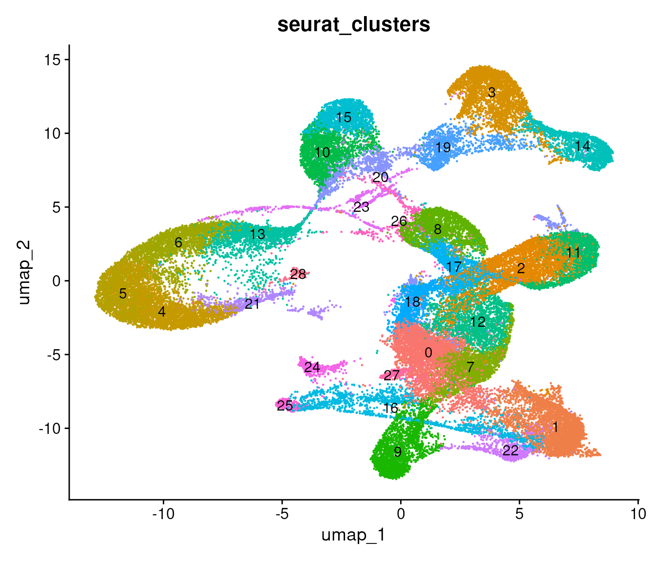
Project the results to all cells
ProjectData() projects the full dataset into the sketch
PCA and UMAP spaces and transfers the sketch cluster labels. We store
the transferred labels as cluster_full and switch back to
the full Atera assay.
The earlier return.model = TRUE saves the UMAP model
needed for this projection. The resulting reductions are
pca.full and full.umap, which let us visualize
all cells using the structure learned from the sketch.
atera_obj <- ProjectData(object = atera_obj,
                        assay = "Atera",
                        sketched.assay = "sketch",
                        sketched.reduction = "pca",
                        full.reduction = "pca.full",
                        dims = 1:10,
                        k.weight = 5,
                        umap.model = "umap",
                        refdata = list(cluster_full = "seurat_clusters"))
## Computing: [========================================] 100% (done)
DefaultAssay(atera_obj) <- "Atera"Visualize clusters
We view both the projected clusters in UMAP space and their locations across the tissue to examine whether an expression group is localized to a tissue compartment or distributed across the sample.
p9 <- DimPlot(atera_obj,
              reduction = "full.umap",
              group.by = "cluster_full",
              label = TRUE) +
              NoLegend() + ggtitle("All cells, projected UMAP")

p9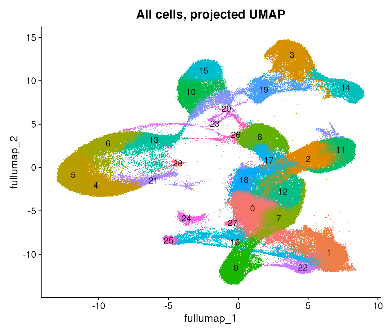
We can color the same projected UMAP by the cell type annotations from Pan-human Azimuth.
DimPlot(atera_obj,
        reduction = "full.umap",
        group.by = "azimuth_broad") + ggtitle("All cells, supplied Azimuth broad cell types")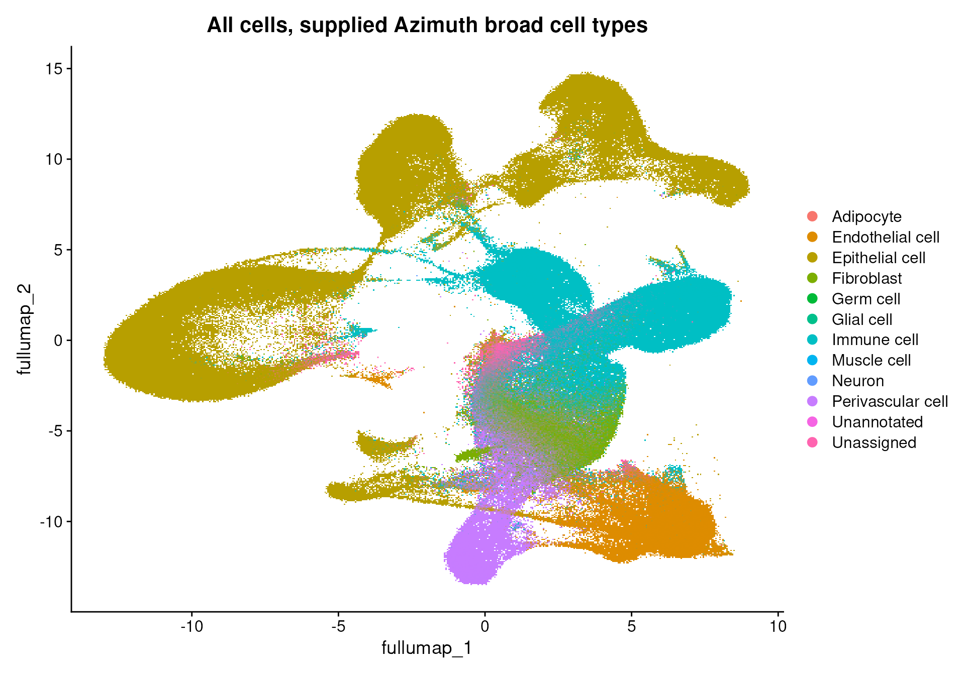
p10 <- ImageDimPlot(atera_obj,
                    fov = "fov",
                    group.by = "cluster_full",
                    size = 0.1) + ggtitle("Clusters, all cells (centroids only)")

p10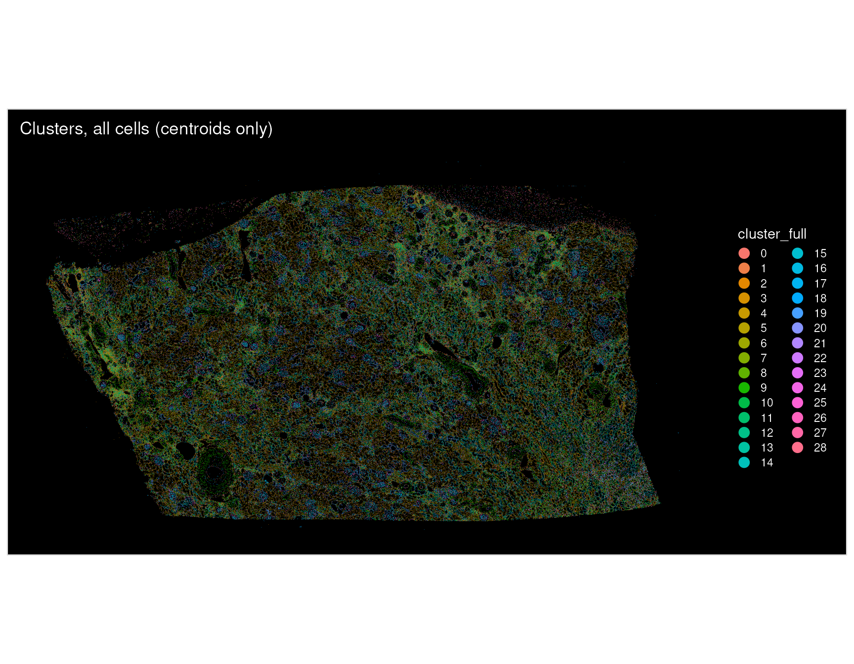
p11 <- ImageDimPlot(atera_obj,
                    fov = "fov.crop",
                    group.by = "cluster_full",
                    boundaries = "segmentations",
                    size = 0.1) + ggtitle("Clusters, cropped region (with cell boundaries)")

p11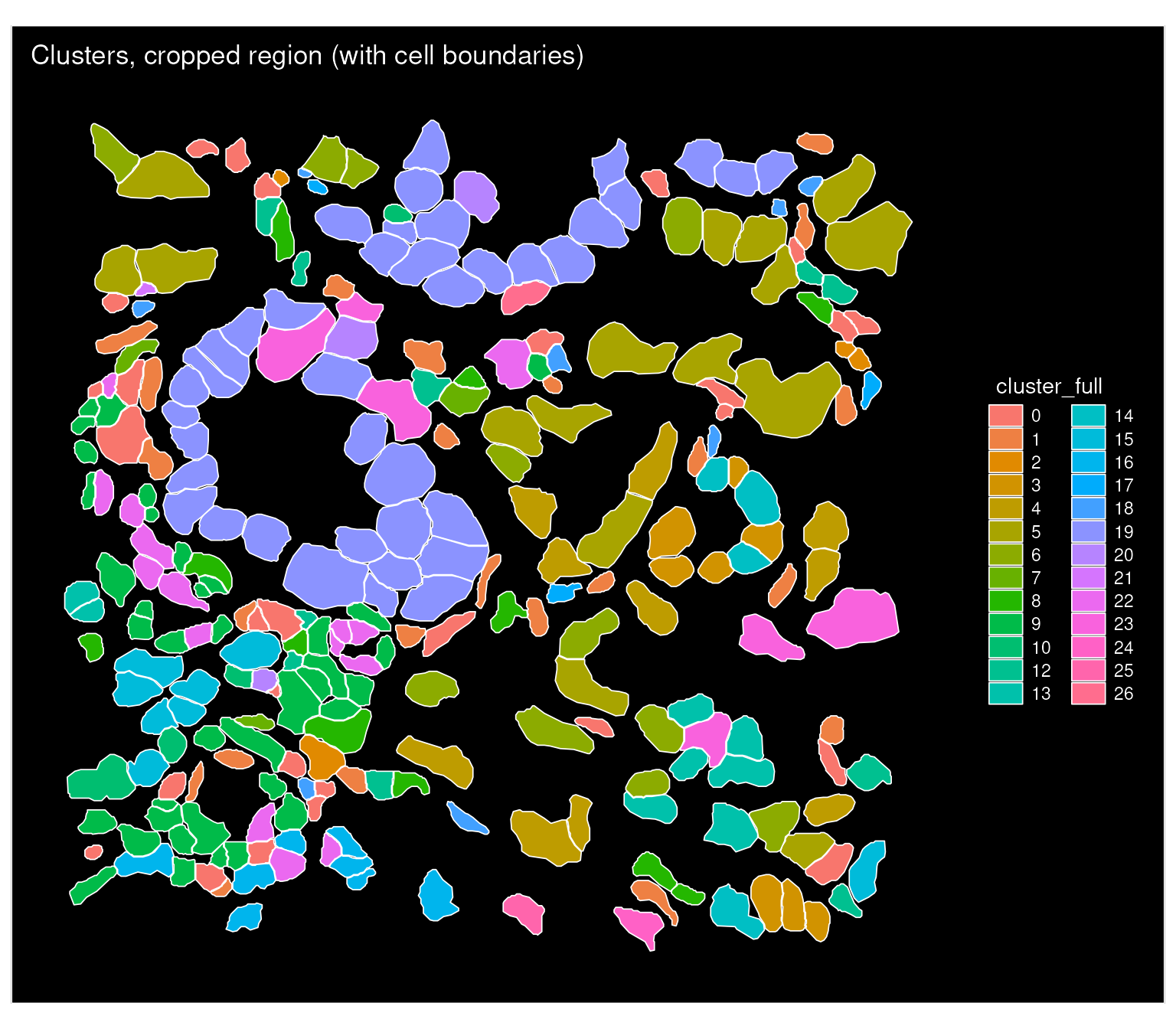
Acknowledgements
We would like to thank Stephen Williams and the Computational Biology team at 10x for their contributions to the code for loading Atera data.
Session Info
sessioninfo::session_info(pkgs = "attached")## ─ Session info ───────────────────────────────────────────────────────────────
## setting value
## version R version 4.5.2 (2025-10-31)
## os Ubuntu 24.04.4 LTS
## system x86_64, linux-gnu
## ui X11
## language en
## collate en_US.UTF-8
## ctype en_US.UTF-8
## tz Etc/UTC
## date 2026-11-06
## pandoc 3.9 @ /usr/bin/ (via rmarkdown)
## quarto 1.8.25 @ /usr/local/bin/quarto
##
## ─ Packages ───────────────────────────────────────────────────────────────────
## package * version date (UTC) lib source
## future * 1.76.0 2026-09-24 [3] CRAN (R 4.5.2)
## ggplot2 * 4.0.3 2026-04-22 [3] CRAN (R 4.5.2)
## magrittr * 2.0.5 2026-04-04 [3] CRAN (R 4.5.2)
## patchwork * 1.3.2 2025-08-25 [3] CRAN (R 4.5.2)
## Seurat * 6.0.0 2026-11-06 [1] local
## SeuratObject * 5.4.0 2026-04-11 [3] RSPM (R 4.5.0)
## sp * 2.2-4 2026-10-11 [3] RSPM (R 4.5.0)
##
## [1] /scratch/build-QLRyQPI9/library
## [2] /usr/local/lib/R/custom-lib
## [3] /usr/local/lib/R/site-library
## [4] /usr/local/lib/R/library
## * ── Packages attached to the search path.
##
## ──────────────────────────────────────────────────────────────────────────────