Analyzing Alternative Polyadenylation in scRNA-seq datasets with PASTA and Seurat
Compiled: June 24, 2024
Source:vignettes/pasta_vignette.Rmd
pasta_vignette.RmdWhile scRNA-seq has been widely applied to characterize cellular heterogeneity in gene expression levels, these datasets can also be leveraged to explore variation in transcript structure as well. For example, reads from 3’ scRNA-seq datasets can be leveraged to quantify the relative usage of multiple polyadenylation (polyA) sites within the same gene.
In Kowalski* , Wessels*, Linder* et al, we introduce a statistical framework, based on the Dirichlet multinomial distribution, to characterize heterogeneity in the relative use of polyA sites at single-cell resolution. We calculate polyA-residuals, which indicate - for each polyA site in each cell - the degree of over or underutilization compared to a background model. We use these residuals for both supervised differential analysis (differential polyadenylation between groups of cells), but also unsupervised analysis and visualization.
We have implemented these methods in an R package PASTA (PolyA Site analysis using relative Transcript Abundance) that interfaces directly with Seurat. In this vignette, we demonstrate how to use PASTA and Seurat to analyze a dataset of 49,958 circulating human peripheral blood mononuclear cells (PBMC). This vignette demonstrates how to reproduce results from Figure 6 in our manuscript. While this represents an initial demonstration of PASTA, we will be adding significant functionality and documentation in future releases.
First, we install PASTA and dependencies.
# install remotes and BiocManager if necessary
if (!requireNamespace("remotes", quietly = TRUE)) install.packages("remotes")
if (!requireNamespace("BiocManager", quietly = TRUE)) install.packages("BiocManager")

# additionally install several Bioconductor dependencies
BiocManager::install(c("BSgenome.Hsapiens.UCSC.hg38", "EnsDb.Hsapiens.v86", "rtracklayer", "GenomicFeatures",
    "plyranges", "org.Hs.eg.db", "clusterProfiler", "enrichplot"))
remotes::install_github("satijalab/PASTA")
# loading PASTA also loads Seurat and Signac
library(PASTA)
library(ggplot2)
library(EnsDb.Hsapiens.v86)
library(org.Hs.eg.db)
library(clusterProfiler)
library(enrichplot)
The data for this vignette can be found on the following site: The files include:
# dir = directory where files are downloaded
counts.file <- paste0(dir, "PBMC_pA_counts.tab.gz")
peak.file <- paste0(dir, "PBMC_polyA_peaks.gff")
fragment.file <- paste0(dir, "PBMC_fragments.tsv.gz")
polyAdb.file <- paste0(dir, "human_PAS_hg38.txt")
metadata.file <- paste0(dir, "PBMC_meta_data.csv")
Create Seurat object and annotate cell types
First, we create a Seurat object based on a pre-quantified scRNA-seq expression matrix of human PBMC. We then annotate cell types using our Azimuth reference, as described here.
library(Azimuth)
counts = Read10X(dir)
pbmc <- CreateSeuratObject(counts, min.cells = 3, min.features = 200)

# add meta data
meta_data <- read.csv(file = metadata.file, row.names = 1)
pbmc <- AddMetaData(pbmc, metadata = meta_data)

# Run Azimuth for each Donor
obj.list <- SplitObject(pbmc, split.by = "donor")
obj.list <- lapply(obj.list, FUN = RunAzimuth, reference = "pbmcref")
pbmc <- merge(obj.list[[1]], obj.list[2:length(obj.list)], merge.dr = "ref.umap")
# note that Azimuth provides higher-resolution annotations with pbmc$celltype.l2
Idents(pbmc) <- pbmc$celltype.l1
library(RColorBrewer)
cols <- colorRampPalette(brewer.pal(8, "Dark2"))(30)
cols.l1 <- cols[c(1:4, 9, 11, 25, 29, 30)]
names(cols.l1) <- c("NK", "CD4 T", "CD8 T", "Other T", "B", "Plasma", "Mono", "DC", "Other")
DimPlot(pbmc, reduction = "ref.umap", label = TRUE, cols = cols.l1)
Adding polyA site counts to the Seurat object
Next, we create a polyA assay that we will add to the Seurat object,
which quantifies the usage (counts) of individual polyA sites in single
cells. PASTA currently accepts polyA site quantifications from the polyApipe
pipeline, but we will be adding support for additional tools in
future releases. The ReadPolyApipe function takes three
input files
- A polyA site count matrix (produced by polyApipe)
- A list of polyA site coordinates (or peaks, also produced by polyApipe)
- A fragment file (produced from the aligned BAM file, we recommend
using the
blocksfunction in sinto.
Once we read in these files, we can create a polyA assay, and add it to the Seurat pbmc object.
options(Seurat.object.assay.calcn = TRUE)
polyA.counts = ReadPolyApipe(counts.file = counts.file, peaks.file = peak.file, filter.chromosomes = TRUE,
    min.features = 10, min.cells = 25)
polyA.assay = CreatePolyAAssay(counts = polyA.counts, genome = "hg38", fragments = fragment.file,
    validate.fragments = FALSE)
# add annotations to polyA.assay
annotations <- GetGRangesFromEnsDb(ensdb = EnsDb.Hsapiens.v86)
genome(annotations) <- "hg38"
Annotation(polyA.assay) <- annotations

# only use cells in both assays
cells = intersect(colnames(pbmc), colnames(polyA.assay))
polyA.assay = subset(polyA.assay, cells = cells)
pbmc = subset(pbmc, cells = cells)
pbmc[["polyA"]] <- polyA.assay  #add polyA assay to Seurat object
DefaultAssay(pbmc) <- "polyA"
pbmc
## An object of class Seurat
## 57907 features across 49958 samples within 5 assays
## Active assay: polyA (41480 features, 0 variable features)
## 2 layers present: counts, data
## 4 other assays present: RNA, prediction.score.celltype.l1, prediction.score.celltype.l2, prediction.score.celltype.l3
## 2 dimensional reductions calculated: integrated_dr, ref.umapAnnotate polyA sites using polyAdbv3
We next annotate each polyA site with information from the PolyA_DB v3
database, which catalogs polyA sites in the human genome based on deep
sequencing data. This GetPolyADbAnnotation function assigns
each polyA site to a gene, and assigns a location within the transcript
(intron, last exon, etc.). This information is stored in the assay, and
can be accessed using the [[]] feature metadata accessor
function.
Note that for polyA sites that receive an NA for the
Gene_Symbol field, these sites did not map to any site
within 50bp in the polyAdbv3 database, and may be spurious.
# max.dist parameter controls maximum distance from polyAdbv3 site
pbmc <- GetPolyADbAnnotation(pbmc, polyAdb.file = polyAdb.file, max.dist = 50)
meta <- pbmc[["polyA"]][[]]
head(meta[, c(1, 13, 15, 18)])
## strand PAS_ID Intron.exon_location
## 10-100000560-100000859 + <NA> <NA>
## 10-100150094-100150393 - chr10:101909851:- 3'_most_exon
## 10-100181533-100181832 - <NA> <NA>
## 10-100188367-100188666 - chr10:101948124:- 3'_most_exon
## 10-100232298-100232597 - chr10:101992055:- 3'_most_exon
## 10-100237155-100237454 - chr10:101996912:- Intron
## Gene_Symbol
## 10-100000560-100000859 <NA>
## 10-100150094-100150393 ERLIN1
## 10-100181533-100181832 <NA>
## 10-100188367-100188666 CHUK
## 10-100232298-100232597 CWF19L1
## 10-100237155-100237454 CWF19L1Quantify relative polyA site usage at single-cell resolution
We can now calculate polyA residuals, as described in our manuscript. For this analysis we will focus on tandem
polyadenylation events reflecting the usage of distinct polyA sites
located in the 3’ UTR of the terminal exon. Once we select features, we
can run the CalcPolyAResiduals function. The residuals are
stored in the scale.data slot of the polyA assay.
# extract features in 3' UTRs
features.last.exon = rownames(subset(meta, Intron.exon_location == "3'_most_exon"))
length(features.last.exon)
## [1] 14985
# gene names are stored in the Gene_Symbol column of the meta features
pbmc <- CalcPolyAResiduals(pbmc, assay = "polyA", features = features.last.exon, gene.names = "Gene_Symbol",
    verbose = TRUE)
Perform dimension reduction on polyA residuals
Now, we can perform dimension reduction directly on the polyA
residuals. The workflow is similar to scRNA-seq: we use
FindVariableFeatures to identify polyA sites that vary
across cells, and then run perform dimension reduction on the variable
polyA sites. We see that there is a very strong separation between
plasma cells and other celltypes.
Plasma cells are known to change their polyA site usage at the IGHM gene, which was one of the first described instances of alternative polydaenylation (Alt et al, Cell, 1980). They have also been shown to change their 3’UTR usage more broadly (Cheng et al, Nature Communications, 2020). Next, we will perform transcriptome-wide analysis to characterize genes whose 3’UTR length changes between plasma cells and B cells.
pbmc <- FindVariableFeatures(pbmc, selection.method = "residuals", gene.names = "Gene_Symbol")
pbmc <- RunPCA(pbmc)
pbmc <- RunUMAP(pbmc, dims = 1:30, reduction.name = "polyA.umap", reduction.key = "polyAUMAP_")
DimPlot(pbmc, group.by = "celltype.l1", reduction = "polyA.umap", cols = cols.l1) + ggtitle("Level 1 Annotations")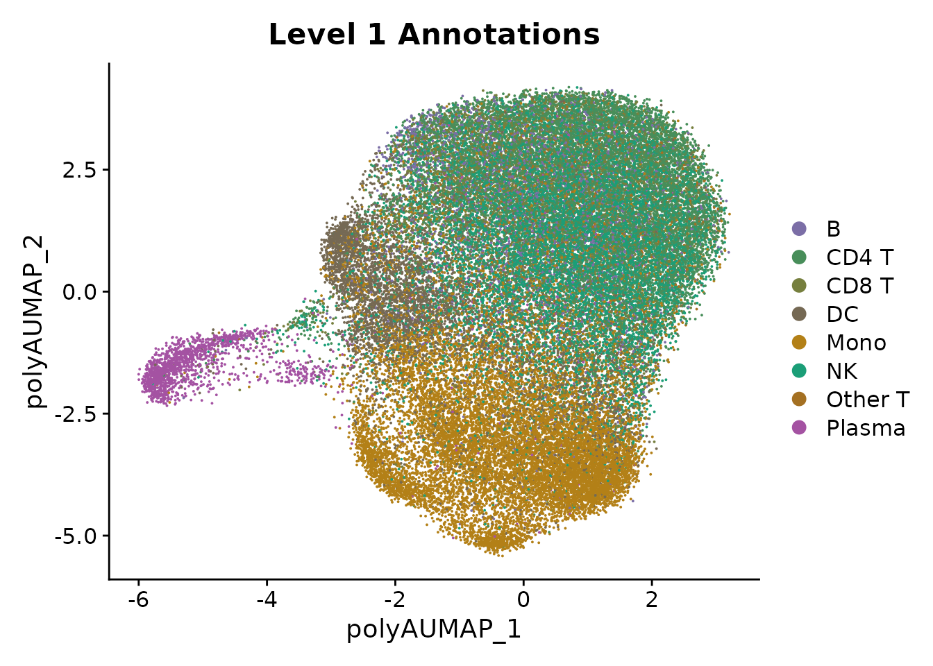
Perform differential polyadenylation analysis
Analagous to differential expression anlaysis, we can also perform differential polyadenylation analysis. As described in our manuscript, this function aims to identify polyA sites whose relative usage within a gene changes across different groups of cells. Here, we identify differentially polyadenylated sites between Plasma cells and B cells.
The FindDifferentialPolyA function returns the following outputs:
- Estimate: Estimated coefficient from the differential APA linear model (indicates the magnitude of change)
- p.value : p-value from the linear model
- p_val_adj: Bonferroni-corrected p-value
- percent.1: The average percent usage (pseudobulk) of the polyA site in the first group of cells
- percent.2: The average percent usage (pseudobulk) of the polyA site in the second group of cells
- symbol: The gene that the polyA site is located in
Idents(pbmc) <- pbmc$celltype.l1
m.plasma <- FindDifferentialPolyA(pbmc, ident.1 = "Plasma", ident.2 = "B", covariates = "donor")
head(m.plasma, 10)
## Estimate p.value p_val_adj percent.1 percent.2
## 12-49762706-49763005 1.1754624 0.000000e+00 0.000000e+00 0.7703972 0.1868293
## 17-41690699-41690998 1.1412147 0.000000e+00 0.000000e+00 0.7710967 0.4299406
## 3-57572076-57572375 1.0510184 0.000000e+00 0.000000e+00 0.7683768 0.2023810
## 6-7882814-7883113 0.6945195 0.000000e+00 0.000000e+00 0.3646308 0.1254658
## 3-57571365-57571664 -0.9942404 0.000000e+00 0.000000e+00 0.2316232 0.7976190
## 17-41691345-41691644 -1.1093621 0.000000e+00 0.000000e+00 0.2264282 0.5646424
## 12-49764635-49764934 -1.1270990 0.000000e+00 0.000000e+00 0.2296028 0.8131707
## 6-7881521-7881820 -0.5560617 1.024656e-290 8.419598e-287 0.6177370 0.8621118
## 18-59327823-59328122 -0.5820680 3.663558e-272 3.010346e-268 0.3585233 0.8545455
## 18-59330929-59331228 0.6292856 1.420368e-269 1.167116e-265 0.6414767 0.1454545
## symbol
## 12-49762706-49763005 TMBIM6
## 17-41690699-41690998 EIF1
## 3-57572076-57572375 ARF4
## 6-7882814-7883113 TXNDC5
## 3-57571365-57571664 ARF4
## 17-41691345-41691644 EIF1
## 12-49764635-49764934 TMBIM6
## 6-7881521-7881820 TXNDC5
## 18-59327823-59328122 LMAN1
## 18-59330929-59331228 LMAN1Visualize polyA site usage across groups of cells
We can also visualize the read coverage across cell groups, which
demonstrates changes in transcript structure across groups of cells. The
PolyACoveragePlot function is based off the
CoveragePlot function in Signac, and uses the previously
computed fragment file to compute local coverage.
Beneath the coverage plot, we also display the location of polyA sites (peaks), as well as gene annotations. Note that in each of these examples, plasma cells exhibit increased utilization of the proximal polyA site (i.e. 3’ UTR shortening).
Idents(pbmc) <- pbmc$celltype.l1
# by default shows all polyAsites where we calculated polyA residuals in a gene
PolyACoveragePlot(pbmc, gene = "EIF1") & scale_fill_manual(values = cols.l1)
PolyACoveragePlot(pbmc, gene = "TMBIM6") & scale_fill_manual(values = cols.l1)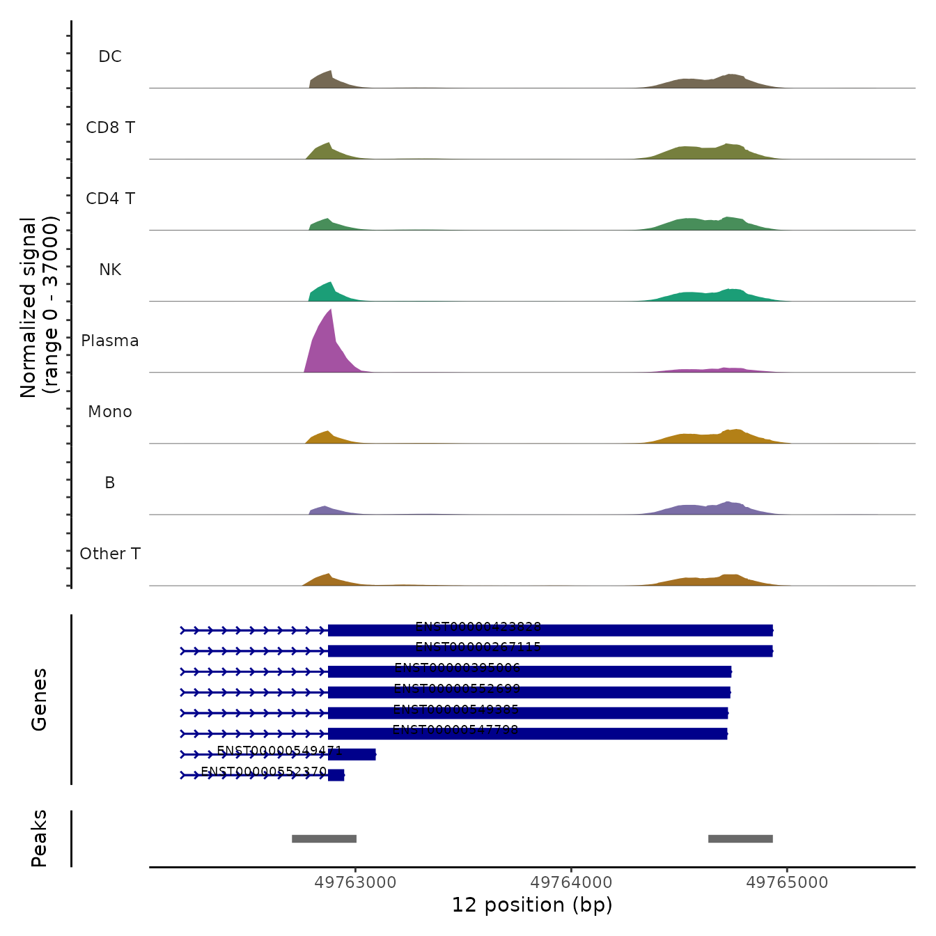
Pathway analysis on genes with changes in 3’UTR length
To understand if the genes that change their 3’UTR usage in plasma cells compared to B cells are enriched in any particular biological process, we perform GO enrichment analysis, as implemented in the clusterProfiler package.
First, we convert the gene symbol of these genes to Entrez IDs, then use the enrichGO function to find pathways that are enriched. Gene Ontology analysis revealed a strong enrichment for Golgi vesicle transport and protein localization, which are linked to the core secretory phenotypes of plasma cells.
plasma.genes <- unique(subset(m.plasma, p_val_adj < 0.05)$symbol)
g.go <- bitr(plasma.genes, fromType = "SYMBOL", toType = "ENTREZID", OrgDb = org.Hs.eg.db)
go.results <- enrichGO(g.go$ENTREZID, "org.Hs.eg.db", ont = "BP", pvalueCutoff = 0.05)
go.results <- setReadable(go.results, OrgDb = org.Hs.eg.db)
go.results.simp <- simplify(go.results, cutoff = 0.7, by = "p.adjust", select_fun = min)
p <- dotplot(go.results.simp)
p + scale_colour_gradient(low = "maroon", high = "grey")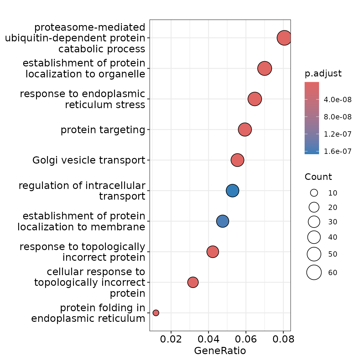
Session Info
## R version 4.3.2 (2023-10-31)
## Platform: x86_64-pc-linux-gnu (64-bit)
## Running under: Ubuntu 20.04.6 LTS
##
## Matrix products: default
## BLAS:   /usr/lib/x86_64-linux-gnu/blas/libblas.so.3.9.0
## LAPACK: /usr/lib/x86_64-linux-gnu/lapack/liblapack.so.3.9.0
##
## locale:
##  [1] LC_CTYPE=en_US.UTF-8       LC_NUMERIC=C
##  [3] LC_TIME=en_US.UTF-8        LC_COLLATE=en_US.UTF-8
##  [5] LC_MONETARY=en_US.UTF-8    LC_MESSAGES=en_US.UTF-8
##  [7] LC_PAPER=en_US.UTF-8       LC_NAME=C
##  [9] LC_ADDRESS=C               LC_TELEPHONE=C
## [11] LC_MEASUREMENT=en_US.UTF-8 LC_IDENTIFICATION=C
##
## time zone: America/New_York
## tzcode source: system (glibc)
##
## attached base packages:
## [1] stats4    stats     graphics  grDevices utils     datasets  methods
## [8] base
##
## other attached packages:
##  [1] RColorBrewer_1.1-3        rlang_1.1.4
##  [3] enrichplot_1.22.0         clusterProfiler_4.10.1
##  [5] org.Hs.eg.db_3.18.0       EnsDb.Hsapiens.v86_2.99.0
##  [7] ensembldb_2.26.0          AnnotationFilter_1.26.0
##  [9] GenomicFeatures_1.54.4    AnnotationDbi_1.64.1
## [11] Biobase_2.62.0            GenomicRanges_1.54.1
## [13] GenomeInfoDb_1.38.8       IRanges_2.36.0
## [15] S4Vectors_0.40.2          BiocGenerics_0.48.1
## [17] ggplot2_3.5.1             PASTA_0.0.0.9000
## [19] Signac_1.13.0             Seurat_5.1.0
## [21] SeuratObject_5.0.2        sp_2.1-4
##
## loaded via a namespace (and not attached):
##   [1] fs_1.6.4                    ProtGenerics_1.34.0
##   [3] matrixStats_1.3.0           spatstat.sparse_3.1-0
##   [5] bitops_1.0-7                HDO.db_0.99.1
##   [7] httr_1.4.7                  backports_1.5.0
##   [9] tools_4.3.2                 sctransform_0.4.1
##  [11] utf8_1.2.4                  R6_2.5.1
##  [13] lazyeval_0.2.2              uwot_0.2.2
##  [15] withr_3.0.0                 prettyunits_1.2.0
##  [17] gridExtra_2.3               progressr_0.14.0
##  [19] MGLM_0.2.1                  cli_3.6.3
##  [21] textshaping_0.4.0           formatR_1.14
##  [23] spatstat.explore_3.2-7      fastDummies_1.7.3
##  [25] scatterpie_0.2.1            sandwich_3.1-0
##  [27] labeling_0.4.3              sass_0.4.9
##  [29] spatstat.data_3.1-2         ggridges_0.5.6
##  [31] pbapply_1.7-2               pkgdown_2.0.7
##  [33] Rsamtools_2.18.0            systemfonts_1.1.0
##  [35] yulab.utils_0.1.4           foreign_0.8-86
##  [37] gson_0.1.0                  R.utils_2.12.3
##  [39] DOSE_3.28.2                 dichromat_2.0-0.1
##  [41] parallelly_1.37.1           BSgenome_1.70.2
##  [43] rstudioapi_0.16.0           RSQLite_2.3.7
##  [45] gridGraphics_0.5-1          generics_0.1.3
##  [47] BiocIO_1.12.0               ica_1.0-3
##  [49] spatstat.random_3.2-3       car_3.1-2
##  [51] dplyr_1.1.4                 GO.db_3.18.0
##  [53] Matrix_1.6-4                fansi_1.0.6
##  [55] abind_1.4-5                 R.methodsS3_1.8.2
##  [57] lifecycle_1.0.4             yaml_2.3.8
##  [59] carData_3.0-5               SummarizedExperiment_1.32.0
##  [61] qvalue_2.34.0               SparseArray_1.2.4
##  [63] BiocFileCache_2.10.2        Rtsne_0.17
##  [65] grid_4.3.2                  blob_1.2.4
##  [67] promises_1.3.0              crayon_1.5.3
##  [69] miniUI_0.1.1.1              lattice_0.22-6
##  [71] cowplot_1.1.3               KEGGREST_1.42.0
##  [73] pillar_1.9.0                knitr_1.47
##  [75] fgsea_1.28.0                rjson_0.2.21
##  [77] future.apply_1.11.2         codetools_0.2-19
##  [79] fastmatch_1.1-4             leiden_0.4.3.1
##  [81] glue_1.7.0                  ggfun_0.1.5
##  [83] data.table_1.15.4           treeio_1.26.0
##  [85] vctrs_0.6.5                 png_0.1-8
##  [87] spam_2.10-0                 gtable_0.3.5
##  [89] cachem_1.1.0                xfun_0.45
##  [91] S4Arrays_1.2.1              mime_0.12
##  [93] tidygraph_1.2.3             survival_3.5-7
##  [95] RcppRoll_0.3.0              fitdistrplus_1.1-11
##  [97] ROCR_1.0-11                 nlme_3.1-165
##  [99] ggtree_3.10.1               bit64_4.0.5
## [101] progress_1.2.3              filelock_1.0.2
## [103] RcppAnnoy_0.0.22            rprojroot_2.0.4
## [105] bslib_0.7.0                 irlba_2.3.5.1
## [107] rpart_4.1.23                KernSmooth_2.23-22
## [109] Hmisc_5.1-3                 colorspace_2.1-0
## [111] DBI_1.2.3                   nnet_7.3-19
## [113] tidyselect_1.2.1            bit_4.0.5
## [115] compiler_4.3.2              curl_5.2.1
## [117] htmlTable_2.4.2             xml2_1.3.6
## [119] desc_1.4.2                  DelayedArray_0.28.0
## [121] plotly_4.10.4               shadowtext_0.1.2
## [123] rtracklayer_1.62.0          checkmate_2.3.1
## [125] scales_1.3.0                lmtest_0.9-40
## [127] rappdirs_0.3.3              stringr_1.5.1
## [129] digest_0.6.36               goftest_1.2-3
## [131] spatstat.utils_3.0-5        rmarkdown_2.27
## [133] XVector_0.42.0              base64enc_0.1-3
## [135] htmltools_0.5.8.1           pkgconfig_2.0.3
## [137] MatrixGenerics_1.14.0       highr_0.11
## [139] dbplyr_2.5.0                fastmap_1.2.0
## [141] htmlwidgets_1.6.4           shiny_1.8.1.1
## [143] farver_2.1.2                jquerylib_0.1.4
## [145] zoo_1.8-12                  jsonlite_1.8.8
## [147] BiocParallel_1.36.0         R.oo_1.26.0
## [149] GOSemSim_2.28.1             VariantAnnotation_1.48.1
## [151] RCurl_1.98-1.14             magrittr_2.0.3
## [153] ggplotify_0.1.2             Formula_1.2-5
## [155] GenomeInfoDbData_1.2.11     dotCall64_1.1-1
## [157] patchwork_1.2.0             munsell_0.5.1
## [159] Rcpp_1.0.12                 ape_5.7-1
## [161] viridis_0.6.5               reticulate_1.38.0
## [163] stringi_1.8.4               ggraph_2.1.0
## [165] zlibbioc_1.48.2             MASS_7.3-60
## [167] plyr_1.8.9                  parallel_4.3.2
## [169] listenv_0.9.1               ggrepel_0.9.5
## [171] deldir_2.0-4                graphlayouts_1.1.1
## [173] Biostrings_2.70.3           splines_4.3.2
## [175] tensor_1.5                  hms_1.1.3
## [177] igraph_2.0.3                spatstat.geom_3.2-9
## [179] RcppHNSW_0.6.0              reshape2_1.4.4
## [181] biomaRt_2.58.2              XML_3.99-0.16.1
## [183] evaluate_0.24.0             biovizBase_1.50.0
## [185] AER_1.2-12                  tweenr_2.0.2
## [187] httpuv_1.6.15               RANN_2.6.1
## [189] tidyr_1.3.1                 purrr_1.0.2
## [191] polyclip_1.10-6             future_1.33.2
## [193] scattermore_1.2             ggforce_0.4.1
## [195] xtable_1.8-4                restfulr_0.0.15
## [197] tidytree_0.4.6              gplm_0.7-4
## [199] RSpectra_0.16-1             later_1.3.2
## [201] viridisLite_0.4.2           ragg_1.3.2
## [203] tibble_3.2.1                aplot_0.2.2
## [205] memoise_2.0.1               plyranges_1.22.0
## [207] GenomicAlignments_1.38.2    cluster_2.1.6
## [209] globals_0.16.3