Pan-human Azimuth in R
This vignette demonstrates how to install and use AzimuthAPI, an
interface for cell type annotation using the Pan-human Azimuth neural
network.
The API takes a Seurat object and returns hierarchical cell type predictions, confidence scores, and low-dimensional embeddings useful for visualization.
Install AzimuthAPI
The Pan-human Azimuth R API, AzimuthAPI, is available for installation
via Github:
remotes::install_github("satijalab/AzimuthAPI")
Load packages & data
library(AzimuthAPI)
library(Seurat)
library(SeuratData)
library(ggplot2)
library(dplyr)
For this vignette, we will demonstrate annotating a dataset of human
bone marrow mononuclear (BMNC) cells that we published as part of
Stuart, Butler et al Cell
2019. This dataset is
available through SeuratData.
bmcite <- InstallData("bmcite")
Load the data from SeuratData. Here we also make sure to normalize the
data before running Pan-human Azimuth.
bmcite <- LoadData("bmcite")
bmcite <- NormalizeData(bmcite)
Annotate a dataset with Pan-human Azimuth
Users have two options for running Pan-human Azimuth on their dataset: cloud-based or local. The cloud-based option is the easiest to use, and requires no additional setup. The local option requires setting up a Python environment with panhumanpy (Python package for the Pan-human Azimuth neural network) and its dependencies.
Annotation results, regardless of the method used, are stored in the Seurat object as cell-level metadata, and the embeddings generated by the underlying neural network are stored in a new Seurat reduction.
Option 1: run CloudAzimuth
The CloudAzimuth function runs Pan-human Azimuth cell type annotation
on a Seurat object via a cloud-based API deployed on AWS.
bmcite_ann <- CloudAzimuth(bmcite)
Option 2: run ANNotate
First, set up a local Python environment:
# Create a new conda environment for Pan-human Azimuth
conda create -n pan-human-azimuth python=3.9
# Activate the environment
conda activate pan-human-azimuth
# Install Pan-human Azimuth and its dependencies
# for more installation options, see https://satijalab.org/pan_human_azimuth/python/panhumanpy.html
pip install panhumanpy
Then ask reticulate to use that environment:
library(reticulate)
# Use the local Python environment for Pan-human Azimuth
use_condaenv("pan-human-azimuth", required = TRUE)
Finally, run the ANNotate function to annotate your dataset. Note that
the initial run may take longer, as the model weights are downloaded and
cached locally.
bmcite_ann <- ANNotate(bmcite)
Examine model output
Pan-human Azimuth returns predictions in multiple formats, as well as softmax probability scores to estimate model confidence.
For more information on the output, see the reference.
# Inspect cell-level metadata returned by the model
md <- bmcite_ann[[]]
# New columns - ex. final_level_labels, final_level_confidence, full_hierarchical_labels -
# have been added to the Seurat object metadata
colnames(md)
##  [1] "orig.ident"                "nCount_RNA"
##  [3] "nFeature_RNA"              "nCount_ADT"
##  [5] "nFeature_ADT"              "lane"
##  [7] "donor"                     "celltype.l1"
##  [9] "celltype.l2"               "RNA.weight"
## [11] "full_hierarchical_labels"  "final_level_labels"
## [13] "final_level_confidence"    "full_consistent_hierarchy"
## [15] "azimuth_broad"             "azimuth_medium"
## [17] "azimuth_fine"              "azimuth_label"
We can view a histogram of softmax probabilities, which reflect the model confidence associated with each cell’s annotation:
ggplot(md, aes(x = final_level_confidence)) + geom_histogram(bins = 20, fill = "skyblue") + labs(x = "Softmax probability",
    y = "Count", title = "Histogram of Softmax Probabilities") + theme_bw()
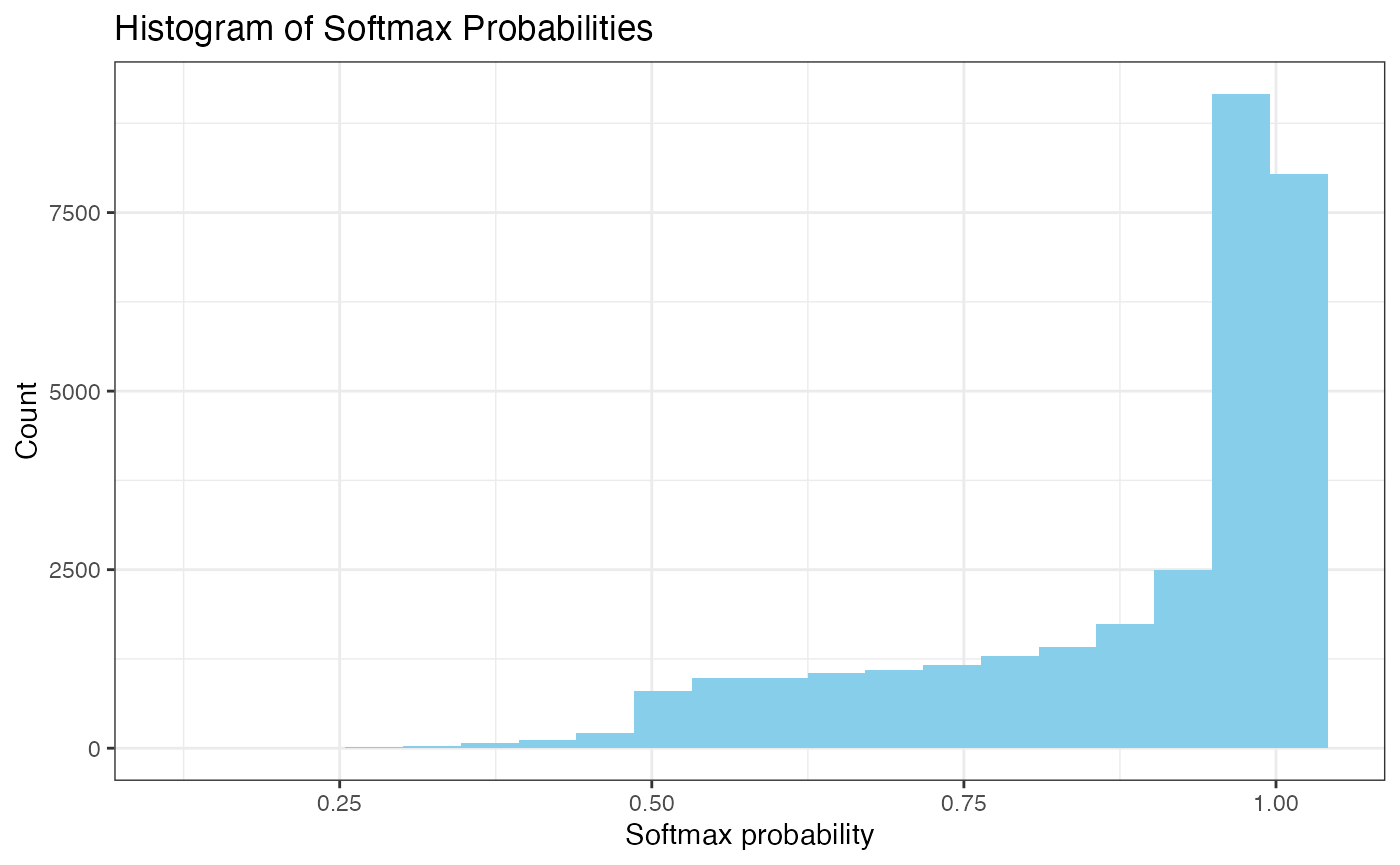
As a QC / filtering step, we can remove cells with low scores:
# remove cells with low scores
bmcite_qc <- subset(bmcite_ann, final_level_confidence > 0.5)
Generate UMAP of Azimuth embeddings
Pan-human Azimuth provides embeddings of the encoding layer generated by
the underlying neural network, stored in the azimuth_embed
128-dimensional reduction. We can use this to generate a two-dimensional
visualization of the dataset, to examine cell type predictions in this
low-dimensional space.
# Use azimuth_embed as input to generate UMAP
bmcite_qc <- RunUMAP(bmcite_qc, dims = 1:128, reduction = "azimuth_embed", reduction.name = "azimuth_umap")
Visualize predictions
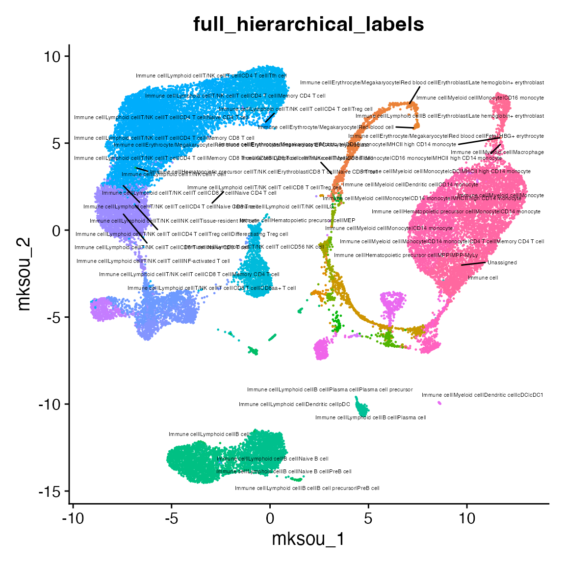
The full_hierarchical_label for each cell provides the model’s classification at each level of granularity, with different levels separated by the ‘|’ character.
p2 <- DimPlot(bmcite_qc, group.by = "full_hierarchical_labels", label.size = 1.5, label = T, reduction = "azimuth_umap",
    repel = TRUE) + NoLegend()
p2
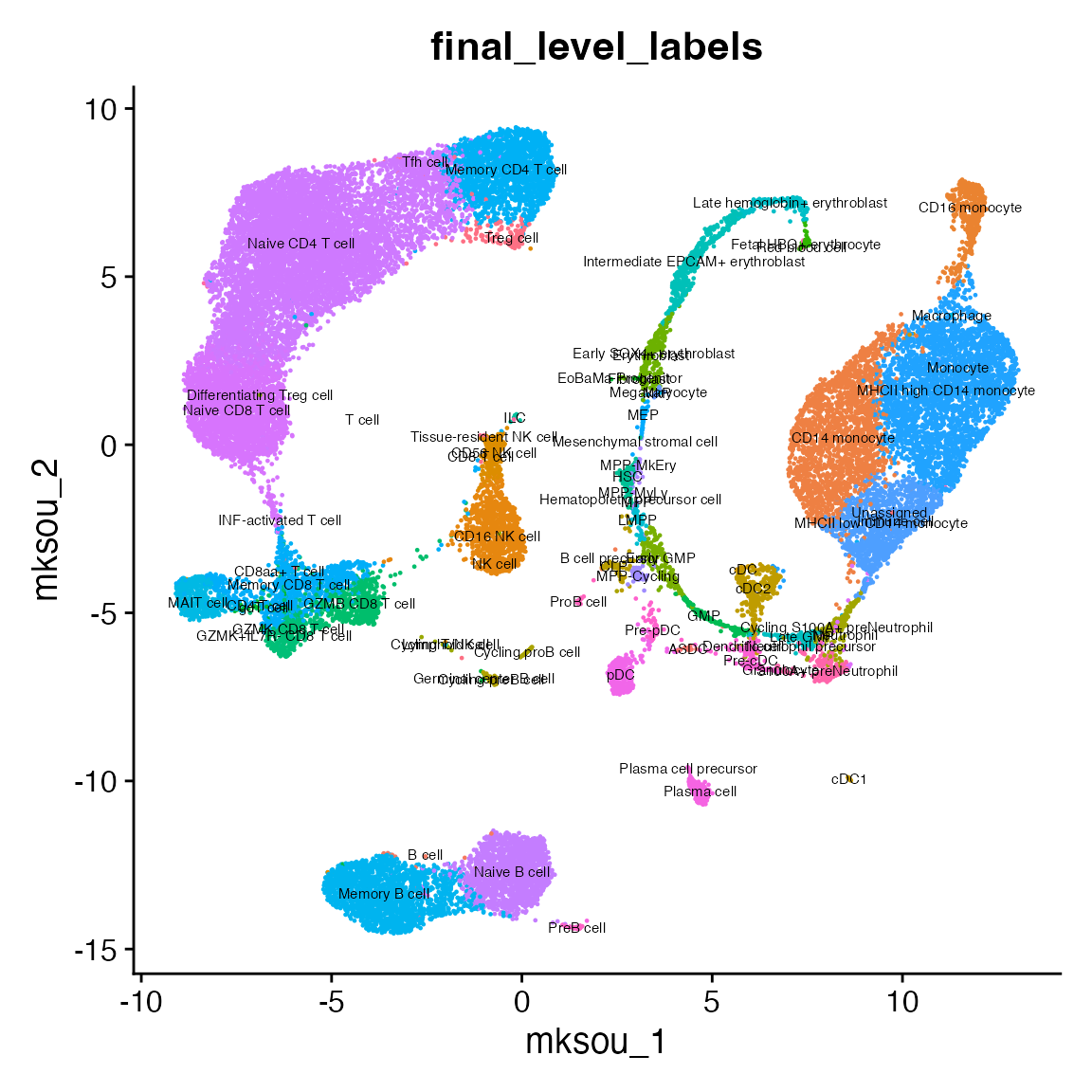
To avoid the long length of the full hierarchical label, we also output
the final level of granularity in a separate column,
final_level_labels, which is the last (most specific)level of the
hierarchy for each cell.
p3 <- DimPlot(bmcite_qc, group.by = "final_level_labels", label.size = 2, label = T, reduction = "azimuth_umap") +
    NoLegend()
p3
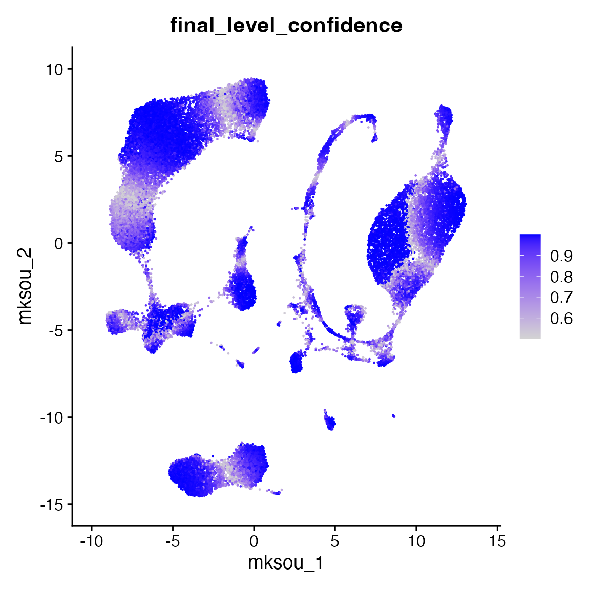
p4 <- FeaturePlot(bmcite_qc, features = "final_level_confidence", reduction = "azimuth_umap")
p4
We also postprocess our predictions to provide labels at three
consistent levels of granularity for easy handling, marking any cell
with an invalid full hierarchical label (based on
full_consistent_hierarchy) as False.
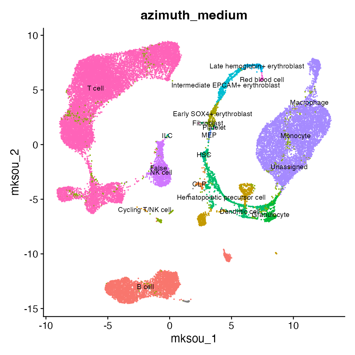
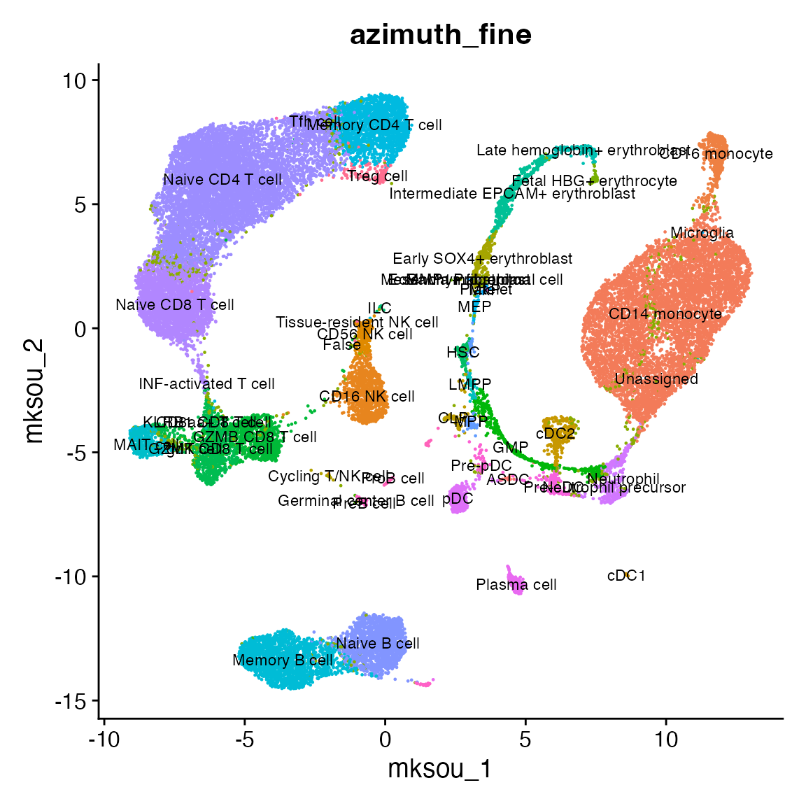
azimuth_broad: Corresponds to level_zero_labels (e.g. Immune cell)azimuth_medium: Medium level of granularity (e.g. T cell)azimuth_fine: High level of granularity (e.g. Treg cell)
These categories provide a consistent level of granularity for each
cell, but may differ from the final_level_label, either by forcing the
model to predict further along the cell type hierarchy than its intial
prediction, or by rolling back its prediction to a lower level of
granularity.
p5 <- DimPlot(bmcite_qc, group.by = "azimuth_medium", label.size = 3, label = T, reduction = "azimuth_umap") +
    NoLegend()
p5
p6 <- DimPlot(bmcite_qc, group.by = "azimuth_fine", label.size = 3, label = T, reduction = "azimuth_umap") +
    NoLegend()
p6
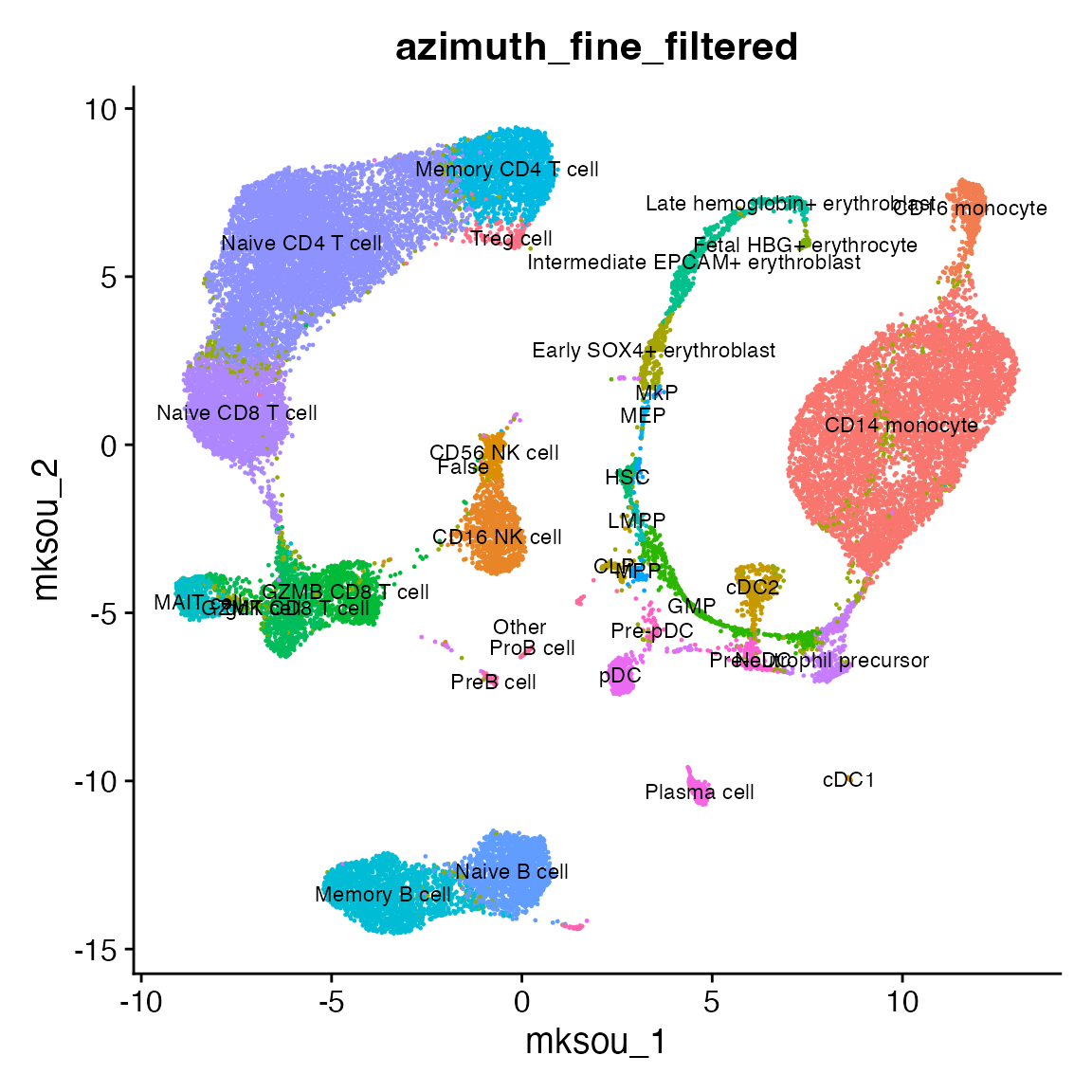
To remove the number of labels displayed, we can filter labels with less
than a certain number of cells using PrepLabel.
Here, we filter labels with less than 20 cells per label. This can be
useful to filter outliers, especially as Pan-human Azimuth does not
perform smoothing of single-cell labels by cluster. Therefore, a single
outlier annotation for one cell will still display the outlier label on
a visualization, and the PrepLabel function can help with this.
bmcite_qc <- PrepLabel(bmcite_qc, "azimuth_fine", "azimuth_fine_filtered", cutoff = 20)
p7 <- DimPlot(bmcite_qc, group.by = "azimuth_fine_filtered", label.size = 3, label = T, reduction = "azimuth_umap") +
    NoLegend()
p7
Visualize differentially expressed features
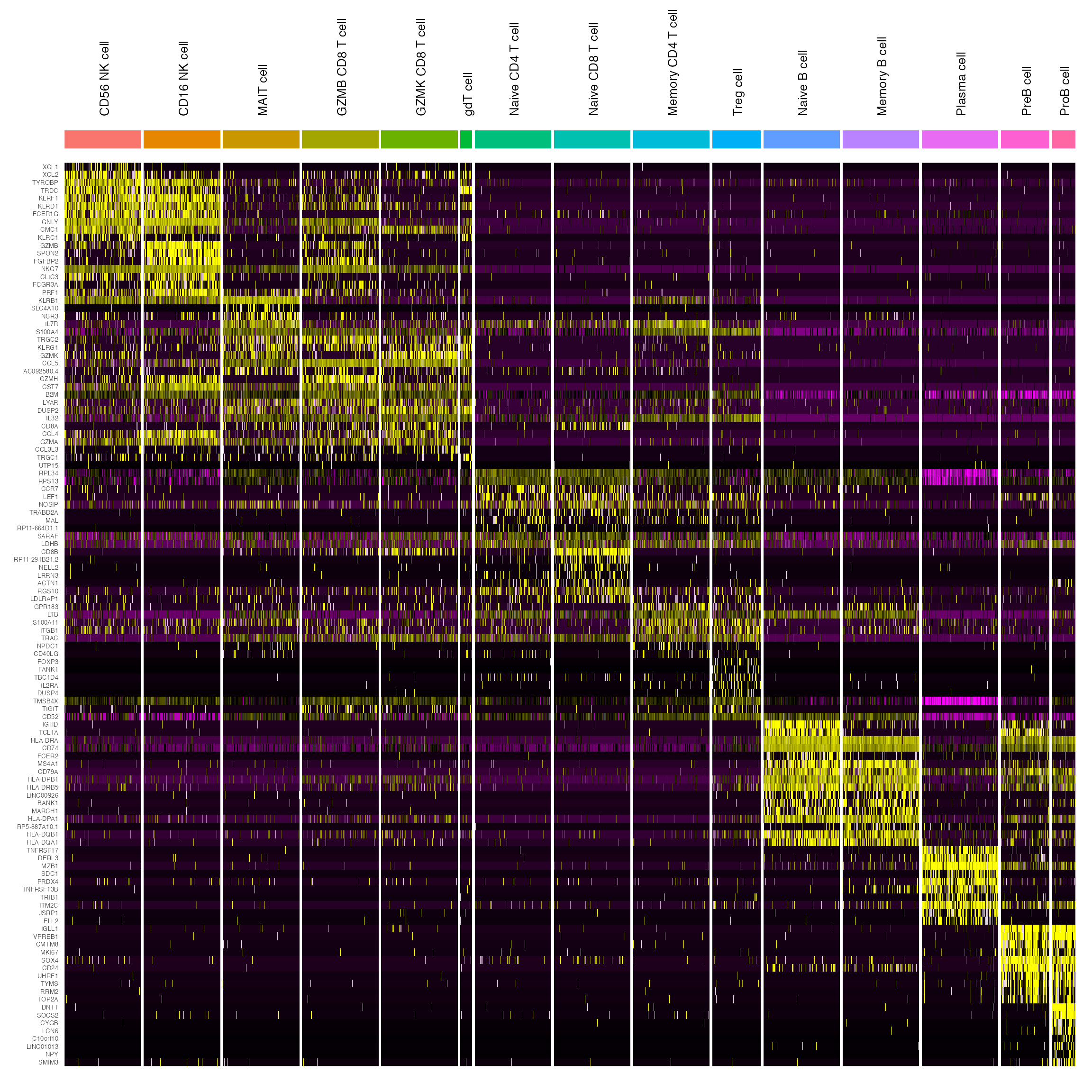
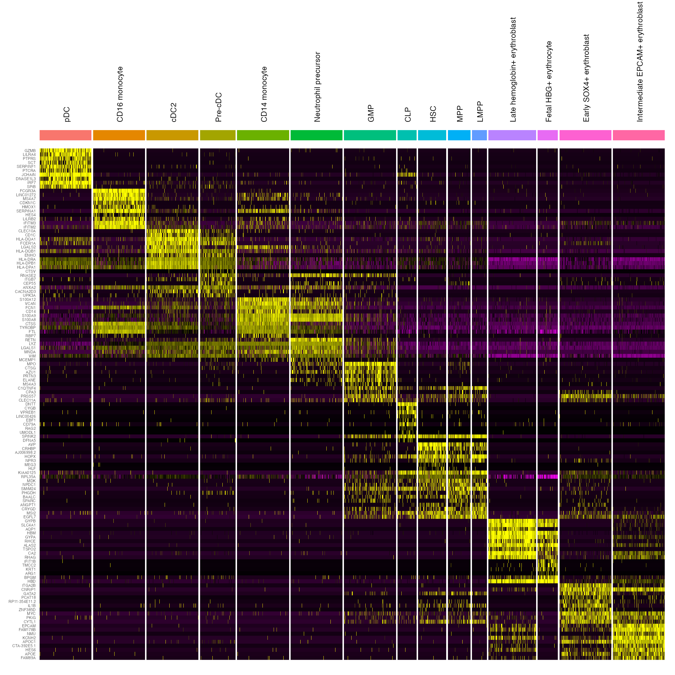
The make_azimuth_QC_heatmaps function allows you to easily explore the
quality of predicted labels by creating expression heatmaps by predicted
cell type, with optional parameters for improved visualization.
Plots are saved by azimuth_broad categories by default, with the
exception of immune cell types grouped separately by lymphoid or
myeloid/erythroid subpopulations.
plots <- make_azimuth_QC_heatmaps(bmcite_qc)
print(length(plots))
## [1] 3
p8 <- plots[["Immune_Lymphoid cell_1"]]
print(p8)
p9 <- plots[["Immune_Myeloid cell_1"]]
print(p9)
More information
For detailed options and usage of the
AzimuthAPIfunctions, see the AzimuthAPI function reference.For another example of the usage of this package, see the Analysis and visualization of Visium HD data with cell segmentations vignette on the Seurat website.
Session Info
sessionInfo()
## R version 4.5.1 (2025-06-13)
## Platform: aarch64-apple-darwin20
## Running under: macOS Sequoia 15.6.1
##
## Matrix products: default
## BLAS:   /Library/Frameworks/R.framework/Versions/4.5-arm64/Resources/lib/libRblas.0.dylib
## LAPACK: /Library/Frameworks/R.framework/Versions/4.5-arm64/Resources/lib/libRlapack.dylib;  LAPACK version 3.12.1
##
## locale:
## [1] en_US.UTF-8/en_US.UTF-8/en_US.UTF-8/C/en_US.UTF-8/en_US.UTF-8
##
## time zone: America/New_York
## tzcode source: internal
##
## attached base packages:
## [1] stats     graphics  grDevices utils     datasets  methods   base
##
## other attached packages:
##  [1] reticulate_1.46.0                dplyr_1.2.1
##  [3] ggplot2_3.5.2                    thp1.eccite.SeuratData_3.1.5
##  [5] stxBrain.SeuratData_0.1.2        ssHippo.SeuratData_3.1.4
##  [7] pbmcsca.SeuratData_3.0.0         pbmcref.SeuratData_1.0.0
##  [9] pbmcMultiome.SeuratData_0.1.4    pbmc3k.SeuratData_3.1.4
## [11] panc8.SeuratData_3.0.2           ifnb.SeuratData_3.1.0
## [13] hcabm40k.SeuratData_3.0.0        celegans.embryo.SeuratData_0.1.0
## [15] cbmc.SeuratData_3.1.4            bmcite.SeuratData_0.3.0
## [17] SeuratData_0.2.2.9002            Seurat_5.5.1
## [19] SeuratObject_5.4.0               sp_2.2-1
## [21] AzimuthAPI_1.0.0
##
## loaded via a namespace (and not attached):
##   [1] RColorBrewer_1.1-3     jsonlite_2.0.0         magrittr_2.0.5
##   [4] spatstat.utils_3.2-3   farver_2.1.2           rmarkdown_2.31
##   [7] fs_2.1.0               ragg_1.4.0             vctrs_0.7.3
##  [10] ROCR_1.0-12            spatstat.explore_3.8-1 RCurl_1.98-1.17
##  [13] htmltools_0.5.9        curl_7.1.0             sass_0.4.10
##  [16] sctransform_0.4.3      parallelly_1.47.0      KernSmooth_2.23-26
##  [19] bslib_0.11.0           htmlwidgets_1.6.4      desc_1.4.3
##  [22] ica_1.0-3              plyr_1.8.9             plotly_4.12.0
##  [25] zoo_1.8-15             cachem_1.1.0           igraph_2.3.3
##  [28] mime_0.13              lifecycle_1.0.5        pkgconfig_2.0.3
##  [31] Matrix_1.7-3           R6_2.6.1               fastmap_1.2.0
##  [34] fitdistrplus_1.2-6     future_1.70.0-9014     shiny_1.14.0
##  [37] digest_0.6.39          patchwork_1.3.2        tensor_1.5.1
##  [40] RSpectra_0.16-2        irlba_2.3.7            textshaping_1.0.1
##  [43] labeling_0.4.3         progressr_0.19.0       spatstat.sparse_3.2-0
##  [46] httr_1.4.8             polyclip_1.10-7        abind_1.4-8
##  [49] compiler_4.5.1         withr_3.0.3            S7_0.2.2
##  [52] fastDummies_1.7.6      argparse_2.3.1         MASS_7.3-65
##  [55] rappdirs_0.3.4         tools_4.5.1            lmtest_0.9-40
##  [58] otel_0.2.0             httpuv_1.6.17          future.apply_1.20.2
##  [61] goftest_1.2-3          glue_1.8.1             nlme_3.1-168
##  [64] promises_1.5.0         grid_4.5.1             Rtsne_0.17
##  [67] cluster_2.1.8.1        reshape2_1.4.5         generics_0.1.4
##  [70] gtable_0.3.6           spatstat.data_3.1-9    tidyr_1.3.2
##  [73] data.table_1.18.4      spatstat.geom_3.8-1    RcppAnnoy_0.0.23
##  [76] ggrepel_0.9.8          RANN_2.6.2             pillar_1.11.1
##  [79] stringr_1.6.0          limma_3.64.3           spam_2.11-4
##  [82] RcppHNSW_0.7.0         later_1.4.8            splines_4.5.1
##  [85] lattice_0.22-7         survival_3.8-3         deldir_2.0-4
##  [88] tidyselect_1.2.1       miniUI_0.1.2           pbapply_1.7-4
##  [91] knitr_1.51             gridExtra_2.3.1        scattermore_1.2
##  [94] xfun_0.59              statmod_1.5.0          matrixStats_1.5.0
##  [97] stringi_1.8.7          lazyeval_0.2.3         yaml_2.3.12
## [100] evaluate_1.0.5         codetools_0.2-20       tibble_3.3.1
## [103] cli_3.6.6              uwot_0.2.4             xtable_1.8-8
## [106] systemfonts_1.2.3      jquerylib_0.1.4        Rcpp_1.1.1-1.1
## [109] globals_0.19.1         spatstat.random_3.5-0  png_0.1-9
## [112] spatstat.univar_3.2-0  parallel_4.5.1         pkgdown_2.2.0
## [115] presto_1.0.0           dotCall64_1.2          bitops_1.0-9
## [118] listenv_1.0.0          viridisLite_0.4.3      scales_1.4.0
## [121] ggridges_0.5.7         purrr_1.2.2            crayon_1.5.3
## [124] rlang_1.2.0            cowplot_1.2.0          formatR_1.14