Introduction to SCTransform, v2 regularization
Compiled: January 17, 2024
Source:vignettes/sctransform_v2_vignette.Rmd
sctransform_v2_vignette.RmdTL;DR
We recently introduced sctransform to perform normalization and variance stabilization of scRNA-seq datasets. We now release an updated version (‘v2’), based on our broad analysis of 59 scRNA-seq datasets spanning a range of technologies, systems, and sequencing depths. This update improves speed and memory consumption, the stability of parameter estimates, the identification of variable features, and the the ability to perform downstream differential expression analyses.
Users can install sctransform v2 from CRAN (sctransform v0.3.3+) and invoke the use of the updated method via the vst.flavor argument.
# install sctransform >= 0.3.3
install.packages("sctransform")
# invoke sctransform - requires Seurat>=4.1
object <- SCTransform(object, vst.flavor = "v2")
Introduction
Heterogeneity in single-cell RNA-seq (scRNA-seq) data is driven by multiple sources, including biological variation in cellular state as well as technical variation introduced during experimental processing. In Choudhary and Satija, 2021 we provide a set of recommendations for modeling variation in scRNA-seq data, particularly when using generalized linear models or likelihood-based approaches for preprocessing and downstream analysis.
In this vignette, we use sctransform v2 based workflow to perform a comparative analysis of human immune cells (PBMC) in either a resting or interferon-stimulated state. In this vignette we apply sctransform-v2 based normalization to perform the following tasks:
- Create an ‘integrated’ data assay for downstream analysis
- Compare the datasets to find cell-type specific responses to stimulation
- Obtain cell type markers that are conserved in both control and stimulated cells
Install sctransform
We will install sctransform v2 from CRAN. We will also install the glmGamPoi package which substantially improves the speed of the learning procedure.
# install glmGamPoi
if (!requireNamespace("BiocManager", quietly = TRUE)) install.packages("BiocManager")
BiocManager::install("glmGamPoi")
# install sctransform from Github
install.packages("sctransform")
Setup the Seurat objects
The dataset is available through our SeuratData package.
# install dataset
InstallData("ifnb")
# load dataset
ifnb <- LoadData("ifnb")

# split the dataset into a list of two seurat objects (stim and CTRL)
ifnb.list <- SplitObject(ifnb, split.by = "stim")

ctrl <- ifnb.list[["CTRL"]]
stim <- ifnb.list[["STIM"]]
Perform normalization and dimensionality reduction
To perform normalization, we invoke SCTransform with an additional flag vst.flavor="v2" to invoke the v2 regularization. This provides some improvements over our original approach first introduced in Hafemeister and Satija, 2019.
- We fix the slope parameter of the GLM to \(\ln(10)\) with \(\log_{10}(\text{total UMI})\) used as the predictor as proposed by Lause et al.
- We utilize an improved parameter estimation procedure that alleviates uncertainty and bias that result from fitting GLM models for very lowly expressed genes.
- We place a lower bound on gene-level standard deviation when calculating Pearson residuals. This prevents genes with extremely low expression (only 1-2 detected UMIs) from having a high pearson residual.
# normalize and run dimensionality reduction on control dataset
ctrl <- SCTransform(ctrl, vst.flavor = "v2", verbose = FALSE) %>%
    RunPCA(npcs = 30, verbose = FALSE) %>%
    RunUMAP(reduction = "pca", dims = 1:30, verbose = FALSE) %>%
    FindNeighbors(reduction = "pca", dims = 1:30, verbose = FALSE) %>%
    FindClusters(resolution = 0.7, verbose = FALSE)

p1 <- DimPlot(ctrl, label = T, repel = T) + ggtitle("Unsupervised clustering")
p2 <- DimPlot(ctrl, label = T, repel = T, group.by = "seurat_annotations") + ggtitle("Annotated celltypes")

p1 | p2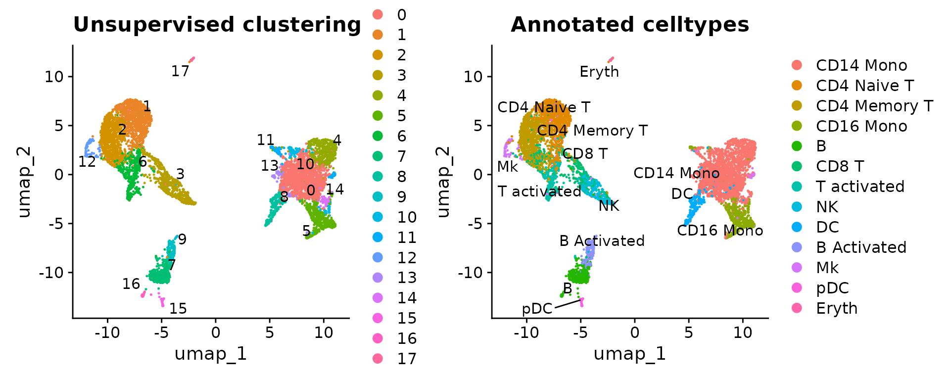
Perform integration using pearson residuals
To perform integration using the pearson residuals calculated above, we use the PrepSCTIntegration() function after selecting a list of informative features using SelectIntegrationFeatures():
stim <- SCTransform(stim, vst.flavor = "v2", verbose = FALSE) %>%
    RunPCA(npcs = 30, verbose = FALSE)
ifnb.list <- list(ctrl = ctrl, stim = stim)
features <- SelectIntegrationFeatures(object.list = ifnb.list, nfeatures = 3000)
ifnb.list <- PrepSCTIntegration(object.list = ifnb.list, anchor.features = features)
To integrate the two datasets, we use the FindIntegrationAnchors() function, which takes a list of Seurat objects as input, and use these anchors to integrate the two datasets together with IntegrateData().
immune.anchors <- FindIntegrationAnchors(object.list = ifnb.list, normalization.method = "SCT",
    anchor.features = features)
immune.combined.sct <- IntegrateData(anchorset = immune.anchors, normalization.method = "SCT")
## [1] 1
## [1] 2Perform an integrated analysis
Now we can run a single integrated analysis on all cells:
immune.combined.sct <- RunPCA(immune.combined.sct, verbose = FALSE)
immune.combined.sct <- RunUMAP(immune.combined.sct, reduction = "pca", dims = 1:30, verbose = FALSE)
immune.combined.sct <- FindNeighbors(immune.combined.sct, reduction = "pca", dims = 1:30)
immune.combined.sct <- FindClusters(immune.combined.sct, resolution = 0.3)
To visualize the two conditions side-by-side, we can use the split.by argument to show each condition colored by cluster.
DimPlot(immune.combined.sct, reduction = "umap", split.by = "stim")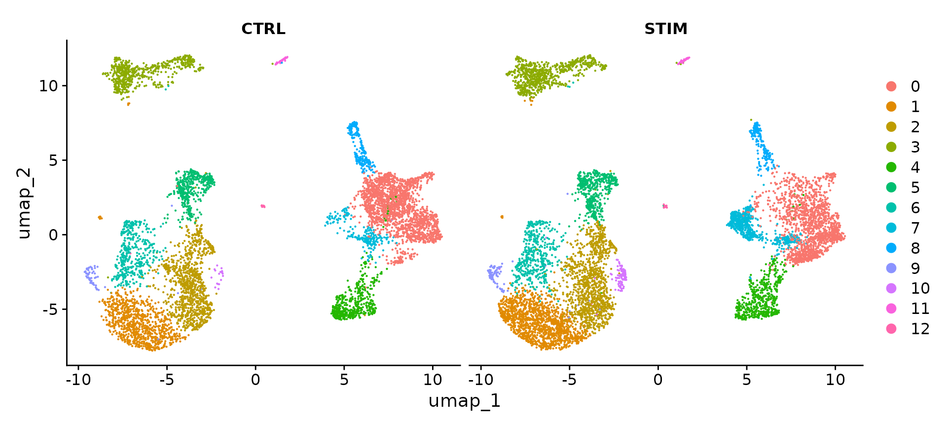
We can also visualize the distribution of annotated celltypes across control and stimulated datasets:
p1 <- DimPlot(immune.combined.sct, reduction = "umap", group.by = "stim")
p2 <- DimPlot(immune.combined.sct, reduction = "umap", group.by = "seurat_clusters", label = TRUE,
    repel = TRUE)
p3 <- DimPlot(immune.combined.sct, reduction = "umap", group.by = "seurat_annotations", label = TRUE,
    repel = TRUE)
p1 | p2 | p3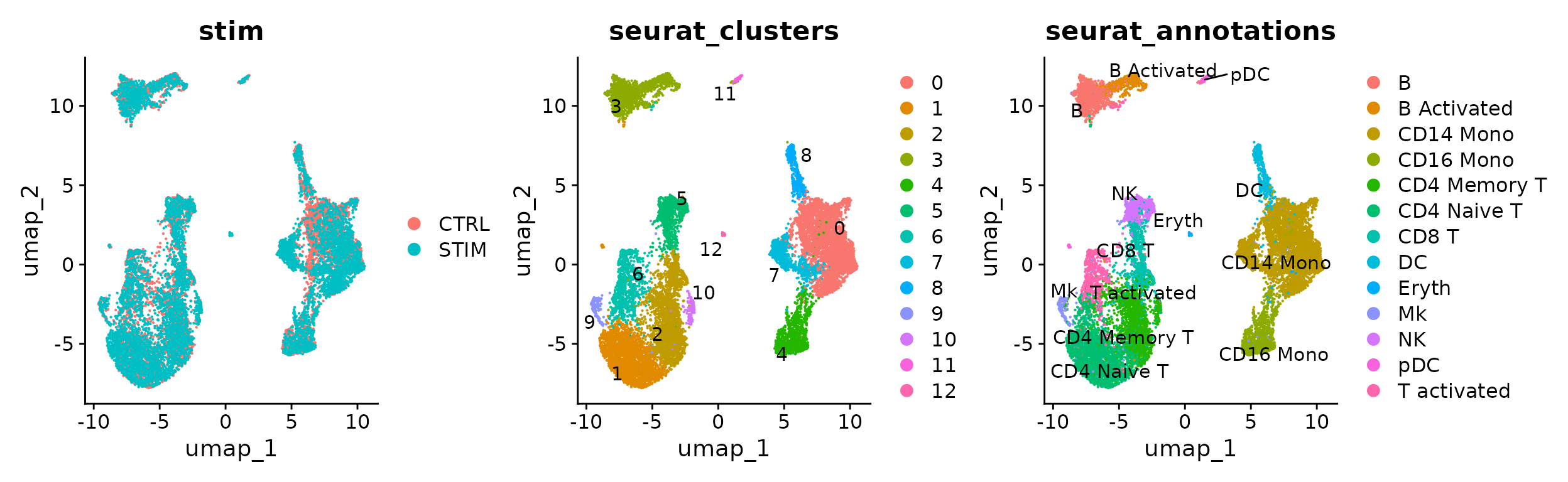
Identify differential expressed genes across conditions
Using the normalized datasets with known celltype annotation, we can ask what genes change in different conditions for cells of the same type. First, we create a column in the meta.data slot to hold both the cell type and stimulation information and switch the current ident to that column.
immune.combined.sct$celltype.stim <- paste(immune.combined.sct$seurat_annotations, immune.combined.sct$stim,
    sep = "_")
Idents(immune.combined.sct) <- "celltype.stim"
To run differential expression, we make use of ‘corrected counts’ that are stored in the data slot of the the SCT assay. Corrected counts are obtained by setting the sequencing depth for all the cells to a fixed value and reversing the learned regularized negative-binomial regression model. Prior to performing differential expression, we first run PrepSCTFindMarkers, which ensures that the fixed value is set properly. Then we use FindMarkers(assay="SCT") to find differentially expressed genes. Here, we aim to identify genes that are differently expressed between stimulated and control B cells.
immune.combined.sct <- PrepSCTFindMarkers(immune.combined.sct)

b.interferon.response <- FindMarkers(immune.combined.sct, assay = "SCT", ident.1 = "B_STIM", ident.2 = "B_CTRL",
    verbose = FALSE)
head(b.interferon.response, n = 15)
## p_val avg_log2FC pct.1 pct.2 p_val_adj
## ISG15 1.505693e-159 5.1598904 0.998 0.229 2.003475e-155
## IFIT3 4.128835e-154 6.2281506 0.961 0.052 5.493827e-150
## IFI6 2.479595e-153 5.6463400 0.965 0.076 3.299349e-149
## ISG20 9.385626e-152 3.1715979 1.000 0.666 1.248851e-147
## IFIT1 2.447118e-139 6.2614957 0.904 0.029 3.256136e-135
## MX1 2.111961e-124 4.1490465 0.900 0.115 2.810175e-120
## LY6E 2.930420e-122 3.9278136 0.898 0.150 3.899217e-118
## TNFSF10 1.104024e-112 6.8254288 0.785 0.020 1.469014e-108
## IFIT2 3.491368e-108 5.5668205 0.783 0.037 4.645615e-104
## B2M 3.405403e-98 0.6074989 1.000 1.000 4.531229e-94
## IRF7 1.114291e-96 3.3721350 0.834 0.187 1.482675e-92
## PLSCR1 3.364901e-96 4.0217697 0.783 0.111 4.477338e-92
## UBE2L6 1.155610e-85 2.6732717 0.849 0.295 1.537655e-81
## CXCL10 5.689834e-84 8.0923962 0.639 0.010 7.570893e-80
## PSMB9 2.304426e-81 1.8684260 0.937 0.568 3.066269e-77If running on a subset of the original object after running PrepSCTFindMarkers(), FindMarkers() should be invoked with recorrect_umi = FALSE to use the existing corrected counts:
immune.combined.sct.subset <- subset(immune.combined.sct, idents = c("B_STIM", "B_CTRL"))
b.interferon.response.subset <- FindMarkers(immune.combined.sct.subset, assay = "SCT", ident.1 = "B_STIM",
    ident.2 = "B_CTRL", verbose = FALSE, recorrect_umi = FALSE)
We can also use the corrected counts for visualization:
Idents(immune.combined.sct) <- "seurat_annotations"
DefaultAssay(immune.combined.sct) <- "SCT"
FeaturePlot(immune.combined.sct, features = c("CD3D", "GNLY", "IFI6"), split.by = "stim", max.cutoff = 3,
    cols = c("grey", "red"))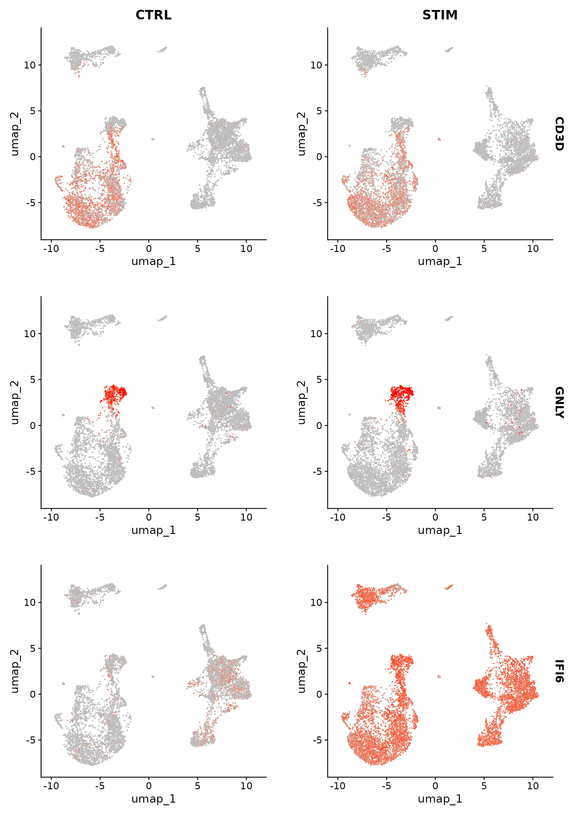
plots <- VlnPlot(immune.combined.sct, features = c("LYZ", "ISG15", "CXCL10"), split.by = "stim",
    group.by = "seurat_annotations", pt.size = 0, combine = FALSE)
wrap_plots(plots = plots, ncol = 1)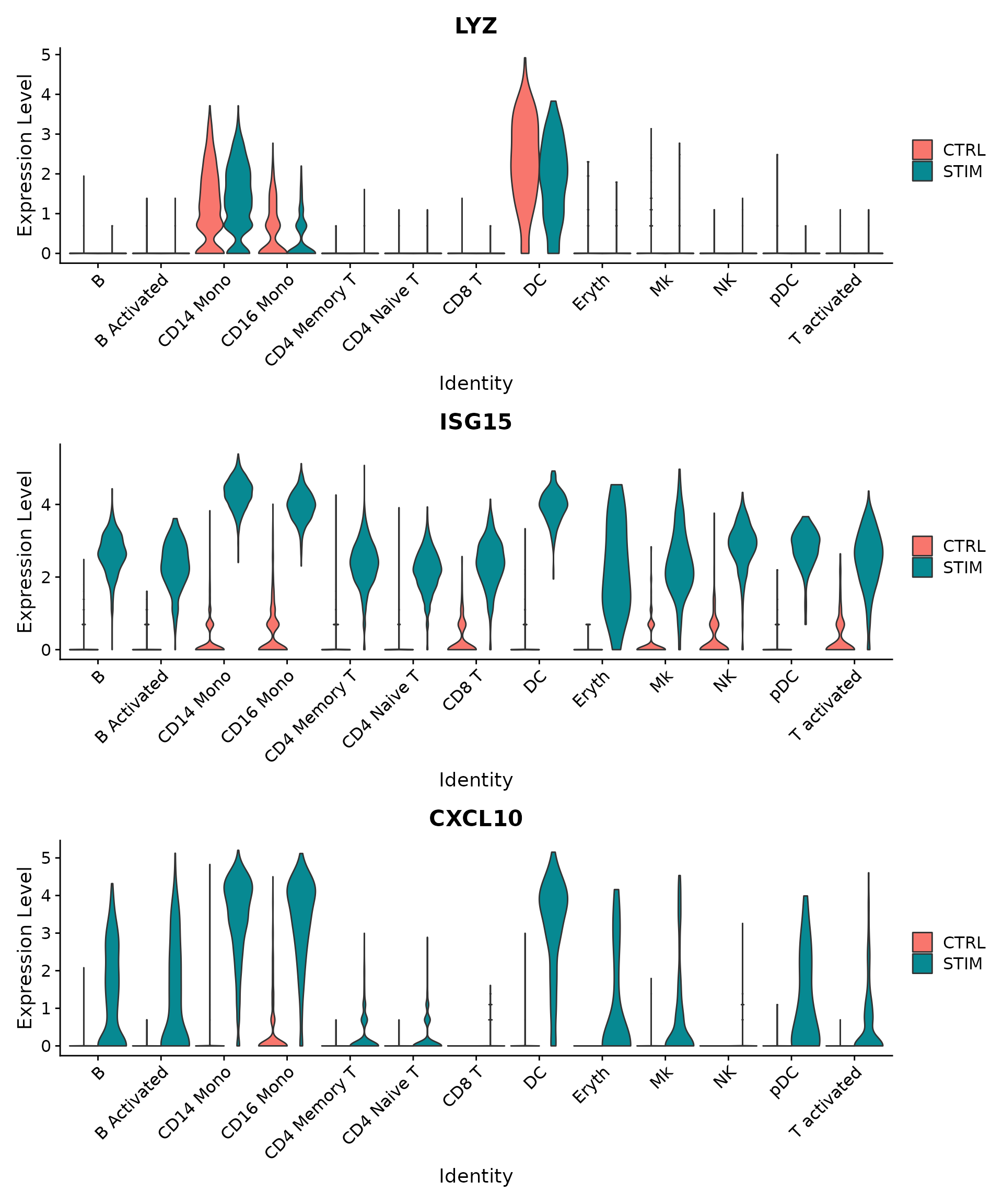
Identify conserved cell type markers
To identify canonical cell type marker genes that are conserved across conditions, we provide the FindConservedMarkers() function. This function performs differential gene expression testing for each dataset/group and combines the p-values using meta-analysis methods from the MetaDE R package. For example, we can identify genes that are conserved markers irrespective of stimulation condition in NK cells. Note that the PrepSCTFindMarkers command does not to be rerun here.
nk.markers <- FindConservedMarkers(immune.combined.sct, assay = "SCT", ident.1 = "NK", grouping.var = "stim",
    verbose = FALSE)
head(nk.markers)
## CTRL_p_val CTRL_avg_log2FC CTRL_pct.1 CTRL_pct.2 CTRL_p_val_adj
## GNLY 0 6.678447 0.943 0.045 0
## NKG7 0 5.190647 0.953 0.080 0
## GZMB 0 4.821619 0.839 0.043 0
## CLIC3 0 5.504544 0.601 0.024 0
## CTSW 0 5.088893 0.537 0.029 0
## KLRD1 0 5.110949 0.507 0.019 0
## STIM_p_val STIM_avg_log2FC STIM_pct.1 STIM_pct.2 STIM_p_val_adj max_pval
## GNLY 0 6.308521 0.956 0.056 0 0
## NKG7 0 4.846749 0.950 0.077 0 0
## GZMB 0 4.958283 0.897 0.058 0 0
## CLIC3 0 5.265345 0.623 0.030 0 0
## CTSW 0 5.099038 0.592 0.035 0 0
## KLRD1 0 4.817659 0.555 0.026 0 0
## minimump_p_val
## GNLY 0
## NKG7 0
## GZMB 0
## CLIC3 0
## CTSW 0
## KLRD1 0Session Info
## R version 4.2.2 Patched (2022-11-10 r83330)
## Platform: x86_64-pc-linux-gnu (64-bit)
## Running under: Ubuntu 20.04.6 LTS
##
## Matrix products: default
## BLAS:   /usr/lib/x86_64-linux-gnu/blas/libblas.so.3.9.0
## LAPACK: /usr/lib/x86_64-linux-gnu/lapack/liblapack.so.3.9.0
##
## locale:
##  [1] LC_CTYPE=en_US.UTF-8       LC_NUMERIC=C
##  [3] LC_TIME=en_US.UTF-8        LC_COLLATE=en_US.UTF-8
##  [5] LC_MONETARY=en_US.UTF-8    LC_MESSAGES=en_US.UTF-8
##  [7] LC_PAPER=en_US.UTF-8       LC_NAME=C
##  [9] LC_ADDRESS=C               LC_TELEPHONE=C
## [11] LC_MEASUREMENT=en_US.UTF-8 LC_IDENTIFICATION=C
##
## attached base packages:
## [1] stats     graphics  grDevices utils     datasets  methods   base
##
## other attached packages:
##  [1] ggplot2_3.4.4                  dplyr_1.1.4
##  [3] patchwork_1.1.3                thp1.eccite.SeuratData_3.1.5
##  [5] stxBrain.SeuratData_0.1.1      ssHippo.SeuratData_3.1.4
##  [7] pbmcsca.SeuratData_3.0.0       pbmcref.SeuratData_1.0.0
##  [9] pbmcMultiome.SeuratData_0.1.4  pbmc3k.SeuratData_3.1.4
## [11] panc8.SeuratData_3.0.2         ifnb.SeuratData_3.0.0
## [13] hcabm40k.SeuratData_3.0.0      cbmc.SeuratData_3.1.4
## [15] bonemarrowref.SeuratData_1.0.0 bmcite.SeuratData_0.3.0
## [17] SeuratData_0.2.2.9001          Seurat_5.0.1.9001
## [19] SeuratObject_5.0.1             sp_2.1-2
##
## loaded via a namespace (and not attached):
##   [1] utf8_1.2.4                  spatstat.explore_3.2-5
##   [3] reticulate_1.34.0           tidyselect_1.2.0
##   [5] htmlwidgets_1.6.4           grid_4.2.2
##   [7] Rtsne_0.17                  munsell_0.5.0
##   [9] mutoss_0.1-13               codetools_0.2-19
##  [11] ragg_1.2.7                  ica_1.0-3
##  [13] future_1.33.0               miniUI_0.1.1.1
##  [15] withr_2.5.2                 spatstat.random_3.2-2
##  [17] colorspace_2.1-0            progressr_0.14.0
##  [19] Biobase_2.58.0              highr_0.10
##  [21] knitr_1.45                  stats4_4.2.2
##  [23] ROCR_1.0-11                 tensor_1.5
##  [25] listenv_0.9.0               Rdpack_2.6
##  [27] MatrixGenerics_1.10.0       labeling_0.4.3
##  [29] GenomeInfoDbData_1.2.9      mnormt_2.1.1
##  [31] polyclip_1.10-6             farver_2.1.1
##  [33] rprojroot_2.0.4             TH.data_1.1-2
##  [35] parallelly_1.36.0           vctrs_0.6.5
##  [37] generics_0.1.3              xfun_0.41
##  [39] R6_2.5.1                    GenomeInfoDb_1.34.9
##  [41] ggbeeswarm_0.7.2            bitops_1.0-7
##  [43] spatstat.utils_3.0-4        cachem_1.0.8
##  [45] DelayedArray_0.24.0         promises_1.2.1
##  [47] scales_1.3.0                multcomp_1.4-25
##  [49] beeswarm_0.4.0              gtable_0.3.4
##  [51] globals_0.16.2              goftest_1.2-3
##  [53] spam_2.10-0                 sandwich_3.1-0
##  [55] rlang_1.1.2                 systemfonts_1.0.5
##  [57] splines_4.2.2               lazyeval_0.2.2
##  [59] spatstat.geom_3.2-7         BiocManager_1.30.22
##  [61] yaml_2.3.8                  reshape2_1.4.4
##  [63] abind_1.4-5                 httpuv_1.6.13
##  [65] tools_4.2.2                 ellipsis_0.3.2
##  [67] jquerylib_0.1.4             RColorBrewer_1.1-3
##  [69] BiocGenerics_0.44.0         ggridges_0.5.5
##  [71] TFisher_0.2.0               Rcpp_1.0.11
##  [73] plyr_1.8.9                  sparseMatrixStats_1.10.0
##  [75] zlibbioc_1.44.0             purrr_1.0.2
##  [77] RCurl_1.98-1.13             deldir_2.0-2
##  [79] pbapply_1.7-2               cowplot_1.1.2
##  [81] S4Vectors_0.36.2            zoo_1.8-12
##  [83] SummarizedExperiment_1.28.0 ggrepel_0.9.4
##  [85] cluster_2.1.6               fs_1.6.3
##  [87] magrittr_2.0.3              data.table_1.14.10
##  [89] RSpectra_0.16-1             glmGamPoi_1.10.2
##  [91] scattermore_1.2             lmtest_0.9-40
##  [93] RANN_2.6.1                  mvtnorm_1.2-4
##  [95] fitdistrplus_1.1-11         matrixStats_1.1.0
##  [97] mime_0.12                   evaluate_0.23
##  [99] xtable_1.8-4                fastDummies_1.7.3
## [101] IRanges_2.32.0              gridExtra_2.3
## [103] compiler_4.2.2              tibble_3.2.1
## [105] KernSmooth_2.23-22          crayon_1.5.2
## [107] htmltools_0.5.7             later_1.3.2
## [109] tidyr_1.3.0                 formatR_1.14
## [111] MASS_7.3-58.2               rappdirs_0.3.3
## [113] Matrix_1.6-4                cli_3.6.2
## [115] rbibutils_2.2.16            qqconf_1.3.2
## [117] metap_1.9                   parallel_4.2.2
## [119] dotCall64_1.1-1             igraph_1.6.0
## [121] GenomicRanges_1.50.2        pkgconfig_2.0.3
## [123] sn_2.1.1                    pkgdown_2.0.7
## [125] numDeriv_2016.8-1.1         plotly_4.10.3
## [127] spatstat.sparse_3.0-3       vipor_0.4.5
## [129] bslib_0.6.1                 multtest_2.54.0
## [131] XVector_0.38.0              stringr_1.5.1
## [133] digest_0.6.33               sctransform_0.4.1
## [135] RcppAnnoy_0.0.21            spatstat.data_3.0-3
## [137] rmarkdown_2.25              leiden_0.4.3.1
## [139] uwot_0.1.16                 DelayedMatrixStats_1.20.0
## [141] shiny_1.8.0                 lifecycle_1.0.4
## [143] nlme_3.1-162                jsonlite_1.8.8
## [145] limma_3.54.2                desc_1.4.2
## [147] viridisLite_0.4.2           fansi_1.0.6
## [149] pillar_1.9.0                lattice_0.21-9
## [151] plotrix_3.8-4               ggrastr_1.0.2
## [153] fastmap_1.1.1               httr_1.4.7
## [155] survival_3.5-7              glue_1.6.2
## [157] png_0.1-8                   presto_1.0.0
## [159] stringi_1.8.3               sass_0.4.8
## [161] textshaping_0.3.7           RcppHNSW_0.5.0
## [163] memoise_2.0.1               mathjaxr_1.6-0
## [165] irlba_2.3.5.1               future.apply_1.11.0