Tips for integrating large datasets
Compiled: 2023-03-27
Source:vignettes/integration_large_datasets.Rmdintegration_large_datasets.RmdFor very large datasets, the standard integration workflow can sometimes be prohibitively computationally expensive. In this workflow, we employ two options that can improve efficiency and runtimes:
- Reciprocal PCA (RPCA)
- Reference-based integration
The main efficiency improvements are gained in FindIntegrationAnchors(). First, we use reciprocal PCA (RPCA) instead of CCA, to identify an effective space in which to find anchors. When determining anchors between any two datasets using reciprocal PCA, we project each dataset into the others PCA space and constrain the anchors by the same mutual neighborhood requirement. All downstream integration steps remain the same and we are able to ‘correct’ (or harmonize) the datasets.
Additionally, we use reference-based integration. In the standard workflow, we identify anchors between all pairs of datasets. While this gives datasets equal weight in downstream integration, it can also become computationally intensive. For example when integrating 10 different datasets, we perform 45 different pairwise comparisons. As an alternative, we introduce here the possibility of specifying one or more of the datasets as the ‘reference’ for integrated analysis, with the remainder designated as ‘query’ datasets. In this workflow, we do not identify anchors between pairs of query datasets, reducing the number of comparisons. For example, when integrating 10 datasets with one specified as a reference, we perform only 9 comparisons. Reference-based integration can be applied to either log-normalized or SCTransform-normalized datasets.
This alternative workflow consists of the following steps:
- Create a list of Seurat objects to integrate
- Perform normalization, feature selection, and scaling separately for each dataset
- Run PCA on each object in the list
- Integrate datasets, and proceed with joint analysis
In general, we observe strikingly similar results between the standard workflow and the one demonstrated here, with substantial reduction in compute time and memory. However, if the datasets are highly divergent (for example, cross-modality mapping or cross-species mapping), where only a small subset of features can be used to facilitate integration, and you may observe superior results using CCA.
For this example, we will be using the “Immune Cell Atlas” data from the Human Cell Atlas which can be found here.
After acquiring the data, we first perform standard normalization and variable feature selection.
bm280k.data <- Read10X_h5("../data/ica_bone_marrow_h5.h5")
bm280k <- CreateSeuratObject(counts = bm280k.data, min.cells = 100, min.features = 500)
bm280k.list <- SplitObject(bm280k, split.by = "orig.ident")
bm280k.list <- lapply(X = bm280k.list, FUN = function(x) {
    x <- NormalizeData(x, verbose = FALSE)
    x <- FindVariableFeatures(x, verbose = FALSE)
})
Next, select features for downstream integration, and run PCA on each object in the list, which is required for running the alternative reciprocal PCA workflow.
features <- SelectIntegrationFeatures(object.list = bm280k.list)
bm280k.list <- lapply(X = bm280k.list, FUN = function(x) {
    x <- ScaleData(x, features = features, verbose = FALSE)
    x <- RunPCA(x, features = features, verbose = FALSE)
})
Since this dataset contains both men and women, we will chose one male and one female (BM1 and BM2) to use in a reference-based workflow. We determined donor sex by examining the expression of the XIST gene.
anchors <- FindIntegrationAnchors(object.list = bm280k.list, reference = c(1, 2), reduction = "rpca",
    dims = 1:50)
bm280k.integrated <- IntegrateData(anchorset = anchors, dims = 1:50)
bm280k.integrated <- ScaleData(bm280k.integrated, verbose = FALSE)
bm280k.integrated <- RunPCA(bm280k.integrated, verbose = FALSE)
bm280k.integrated <- RunUMAP(bm280k.integrated, dims = 1:50)
DimPlot(bm280k.integrated, group.by = "orig.ident")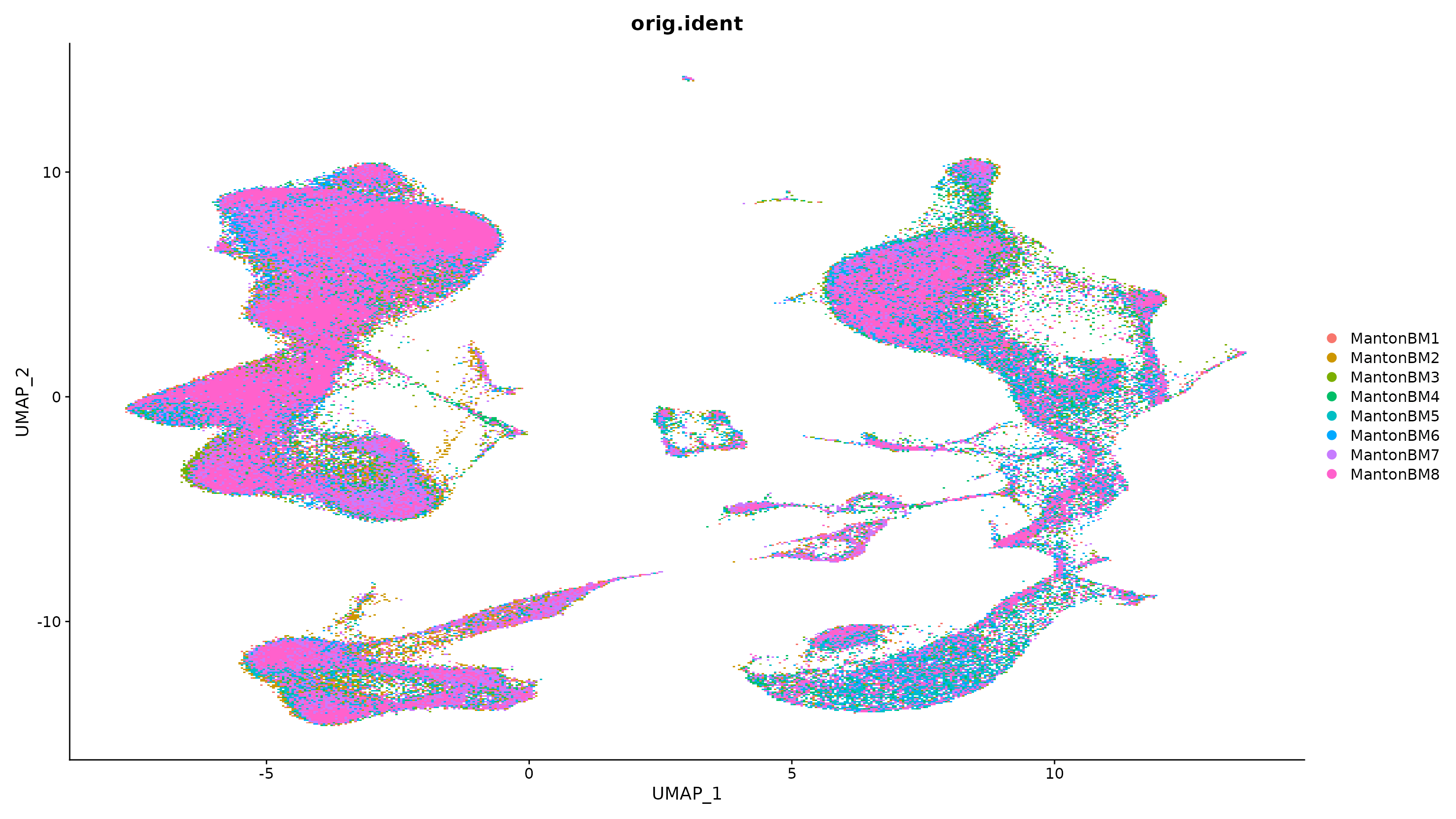
Session Info
## R version 4.2.0 (2022-04-22)
## Platform: x86_64-pc-linux-gnu (64-bit)
## Running under: Ubuntu 20.04.5 LTS
##
## Matrix products: default
## BLAS:   /usr/lib/x86_64-linux-gnu/openblas-pthread/libblas.so.3
## LAPACK: /usr/lib/x86_64-linux-gnu/openblas-pthread/liblapack.so.3
##
## locale:
##  [1] LC_CTYPE=en_US.UTF-8       LC_NUMERIC=C
##  [3] LC_TIME=en_US.UTF-8        LC_COLLATE=en_US.UTF-8
##  [5] LC_MONETARY=en_US.UTF-8    LC_MESSAGES=en_US.UTF-8
##  [7] LC_PAPER=en_US.UTF-8       LC_NAME=C
##  [9] LC_ADDRESS=C               LC_TELEPHONE=C
## [11] LC_MEASUREMENT=en_US.UTF-8 LC_IDENTIFICATION=C
##
## attached base packages:
## [1] stats     graphics  grDevices utils     datasets  methods   base
##
## other attached packages:
## [1] ggplot2_3.4.1      SeuratObject_4.1.3 Seurat_4.3.0
##
## loaded via a namespace (and not attached):
##   [1] Rtsne_0.16             colorspace_2.1-0       deldir_1.0-6
##   [4] ellipsis_0.3.2         ggridges_0.5.4         rprojroot_2.0.3
##   [7] fs_1.6.1               spatstat.data_3.0-0    farver_2.1.1
##  [10] leiden_0.4.3           listenv_0.9.0          bit64_4.0.5
##  [13] ggrepel_0.9.3          fansi_1.0.4            codetools_0.2-18
##  [16] splines_4.2.0          cachem_1.0.7           knitr_1.42
##  [19] polyclip_1.10-4        jsonlite_1.8.4         ica_1.0-3
##  [22] cluster_2.1.3          png_0.1-8              uwot_0.1.14
##  [25] spatstat.sparse_3.0-0  shiny_1.7.4            sctransform_0.3.5
##  [28] compiler_4.2.0         httr_1.4.5             Matrix_1.5-3
##  [31] fastmap_1.1.1          lazyeval_0.2.2         cli_3.6.0
##  [34] later_1.3.0            formatR_1.14           htmltools_0.5.4
##  [37] tools_4.2.0            igraph_1.4.1           gtable_0.3.1
##  [40] glue_1.6.2             RANN_2.6.1             reshape2_1.4.4
##  [43] dplyr_1.1.0            Rcpp_1.0.10            scattermore_0.8
##  [46] jquerylib_0.1.4        pkgdown_2.0.7          vctrs_0.5.2
##  [49] nlme_3.1-157           spatstat.explore_3.0-6 progressr_0.13.0
##  [52] lmtest_0.9-40          spatstat.random_3.1-3  xfun_0.37
##  [55] stringr_1.5.0          globals_0.16.2         mime_0.12
##  [58] miniUI_0.1.1.1         lifecycle_1.0.3        irlba_2.3.5.1
##  [61] goftest_1.2-3          future_1.31.0          MASS_7.3-56
##  [64] zoo_1.8-11             scales_1.2.1           ragg_1.2.5
##  [67] promises_1.2.0.1       spatstat.utils_3.0-1   parallel_4.2.0
##  [70] RColorBrewer_1.1-3     yaml_2.3.7             memoise_2.0.1
##  [73] reticulate_1.28        pbapply_1.7-0          gridExtra_2.3
##  [76] sass_0.4.5             stringi_1.7.12         highr_0.10
##  [79] desc_1.4.2             rlang_1.0.6            pkgconfig_2.0.3
##  [82] systemfonts_1.0.4      matrixStats_0.63.0     evaluate_0.20
##  [85] lattice_0.20-45        tensor_1.5             ROCR_1.0-11
##  [88] purrr_1.0.1            labeling_0.4.2         patchwork_1.1.2
##  [91] htmlwidgets_1.6.1      bit_4.0.5              cowplot_1.1.1
##  [94] tidyselect_1.2.0       parallelly_1.34.0      RcppAnnoy_0.0.20
##  [97] plyr_1.8.8             magrittr_2.0.3         R6_2.5.1
## [100] generics_0.1.3         withr_2.5.0            pillar_1.8.1
## [103] fitdistrplus_1.1-8     abind_1.4-5            survival_3.3-1
## [106] sp_1.6-0               tibble_3.1.8           future.apply_1.10.0
## [109] hdf5r_1.3.8            KernSmooth_2.23-20     utf8_1.2.3
## [112] spatstat.geom_3.0-6    plotly_4.10.1          rmarkdown_2.20
## [115] grid_4.2.0             data.table_1.14.8      digest_0.6.31
## [118] xtable_1.8-4           tidyr_1.3.0            httpuv_1.6.9
## [121] textshaping_0.3.6      munsell_0.5.0          viridisLite_0.4.1
## [124] bslib_0.4.2