Seurat - Dimensional Reduction Vignette
Compiled: March 27, 2023
Source:vignettes/dim_reduction_vignette.Rmddim_reduction_vignette.RmdLoad in the data
This vignette demonstrates how to store and interact with dimensional reduction information (such as the output from RunPCA()) in Seurat. For demonstration purposes, we will be using the 2,700 PBMC object that is available via the SeuratData package.
library(Seurat)
library(SeuratData)
pbmc <- LoadData("pbmc3k", type = "pbmc3k.final")
Explore the new dimensional reduction structure
In Seurat v3.0, storing and interacting with dimensional reduction information has been generalized and formalized into the DimReduc object. Each dimensional reduction procedure is stored as a DimReduc object in the object@reductions slot as an element of a named list. Accessing these reductions can be done with the [[ operator, calling the name of the reduction desired. For example, after running a principle component analysis with RunPCA(), object[['pca']] will contain the results of the PCA. By adding new elements to the list, users can add additional, and custom, dimensional reductions. Each stored dimensional reduction contains the following slots:
- cell.embeddings: stores the coordinates for each cell in low-dimensional space.
- feature.loadings: stores the weight for each feature along each dimension of the embedding
- feature.loadings.projected: Seurat typically calculate the dimensional reduction on a subset of genes (for example, high-variance genes), and then project that structure onto the entire dataset (all genes). The results of that projection (calculated with
ProjectDim()) are stored in this slot. Note that the cell loadings will remain unchanged after projection but there are now feature loadings for all feature - stdev: The standard deviations of each dimension. Most often used with PCA (storing the square roots of the eigenvalues of the covariance matrix) and can be useful when looking at the drop off in the amount of variance that is explained by each successive dimension.
- key: Sets the column names for the cell.embeddings and feature.loadings matrices. For example, for PCA, the column names are PC1, PC2, etc., so the key is “PC”.
- jackstraw: Stores the results of the jackstraw procedure run using this dimensional reduction technique. Currently supported only for PCA.
- misc: Bonus slot to store any other information you might want
To access these slots, we provide the Embeddings(),Loadings(), and Stdev() functions
pbmc[["pca"]]## A dimensional reduction object with key PC_
## Number of dimensions: 50
## Projected dimensional reduction calculated: FALSE
## Jackstraw run: TRUE
## Computed using assay: RNA
head(Embeddings(pbmc, reduction = "pca")[, 1:5])## PC_1 PC_2 PC_3 PC_4 PC_5
## AAACATACAACCAC -4.7296855 -0.5184265 -0.7623220 -2.3156790 -0.07160006
## AAACATTGAGCTAC -0.5174029 4.5918957 5.9091921 6.9118856 -1.96243034
## AAACATTGATCAGC -3.1891063 -3.4695154 -0.8313710 -2.0019985 -5.10442765
## AAACCGTGCTTCCG 12.7933021 0.1007166 0.6310221 -0.3687338 0.21838204
## AAACCGTGTATGCG -3.1288078 -6.3481412 1.2507776 3.0191026 7.84739502
## AAACGCACTGGTAC -3.1088963 0.9262125 -0.6482331 -2.3244378 -2.00526763## PC_1 PC_2 PC_3 PC_4 PC_5
## PPBP 0.010990202 0.01148426 -0.15176092 0.10403737 0.003299077
## LYZ 0.116231706 0.01472515 -0.01280613 -0.04414540 0.049906881
## S100A9 0.115414362 0.01895146 -0.02368853 -0.05787777 0.085382309
## IGLL5 -0.007987473 0.05454239 0.04901533 0.06694722 0.004603231
## GNLY -0.015238762 -0.13375626 0.04101340 0.06912322 0.104558611
## FTL 0.118292572 0.01871142 -0.00984755 -0.01555269 0.038743505## [1] 7.098420 4.495493 3.872592 3.748859 3.171755 2.545292Seurat provides RunPCA() (pca), and RunTSNE() (tsne), and representing dimensional reduction techniques commonly applied to scRNA-seq data. When using these functions, all slots are filled automatically.
We also allow users to add the results of a custom dimensional reduction technique (for example, multi-dimensional scaling (MDS), or zero-inflated factor analysis), that is computed separately. All you need is a matrix with each cell’s coordinates in low-dimensional space, as shown below.
Storing a custom dimensional reduction calculation
Though not incorporated as part of the Seurat package, its easy to run multidimensional scaling (MDS) in R. If you were interested in running MDS and storing the output in your Seurat object:
# Before running MDS, we first calculate a distance matrix between all pairs of cells.  Here
# we use a simple euclidean distance metric on all genes, using scale.data as input
d <- dist(t(GetAssayData(pbmc, slot = "scale.data")))
# Run the MDS procedure, k determines the number of dimensions
mds <- cmdscale(d = d, k = 2)
# cmdscale returns the cell embeddings, we first label the columns to ensure downstream
# consistency
colnames(mds) <- paste0("MDS_", 1:2)
# We will now store this as a custom dimensional reduction called 'mds'
pbmc[["mds"]] <- CreateDimReducObject(embeddings = mds, key = "MDS_", assay = DefaultAssay(pbmc))

# We can now use this as you would any other dimensional reduction in all downstream functions
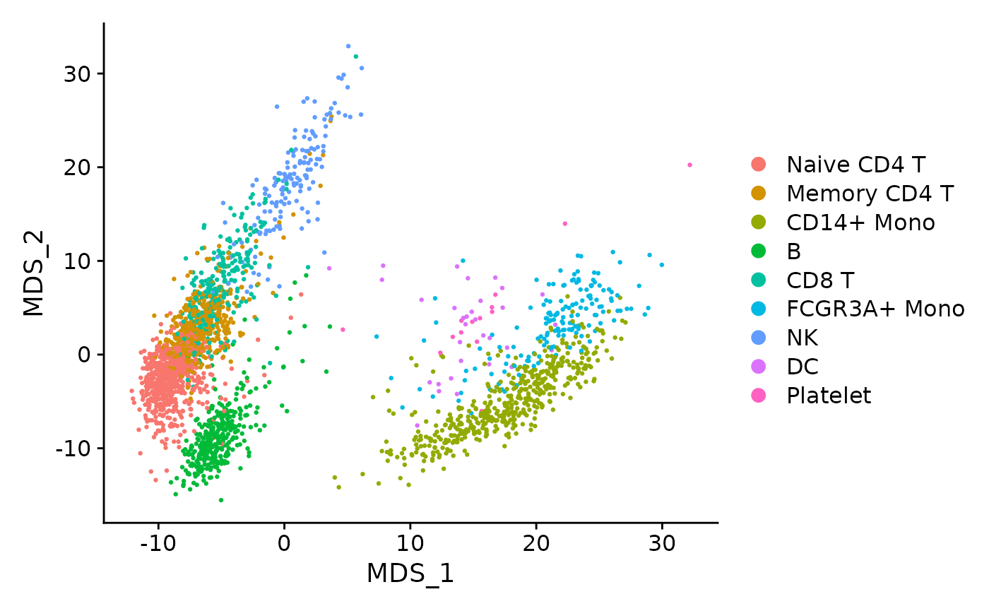
DimPlot(pbmc, reduction = "mds", pt.size = 0.5)
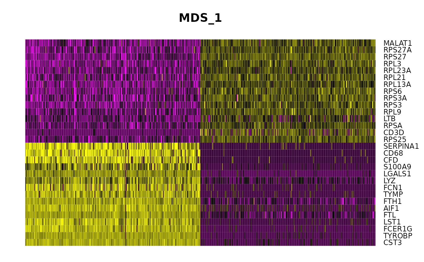
# If you wold like to observe genes that are strongly correlated with the first MDS coordinate
pbmc <- ProjectDim(pbmc, reduction = "mds")
## MDS_ 1
## Positive: CST3, TYROBP, FCER1G, LST1, FTL, AIF1, FTH1, TYMP, FCN1, LYZ
## LGALS1, S100A9, CFD, CD68, SERPINA1, CTSS, IFITM3, SPI1, S100A8, LGALS2
## Negative: MALAT1, RPS27A, RPS27, RPL3, RPL23A, RPL21, RPL13A, RPS6, RPS3A, RPS3
## RPL9, LTB, RPSA, CD3D, RPS25, RPS18, PTPRCAP, RPS12, RPL30, RPL31
## MDS_ 2
## Positive: NKG7, PRF1, CST7, GZMA, GZMB, B2M, FGFBP2, CTSW, GNLY, HLA-C
## GZMH, SPON2, CD247, FCGR3A, CCL5, HLA-A, CCL4, GZMM, KLRD1, CLIC3
## Negative: RPL32, RPL18A, HLA-DRA, CD79A, RPL13, MS4A1, RPL11, TCL1A, RPS9, RPL12
## LINC00926, HLA-DQB1, HLA-DQA1, HLA-DRB1, RPL28, RPS2, S100A8, HLA-DMA, RPL8, RPLP1
# Display the results as a heatmap
DimHeatmap(pbmc, reduction = "mds", dims = 1, cells = 500, projected = TRUE, balanced = TRUE)
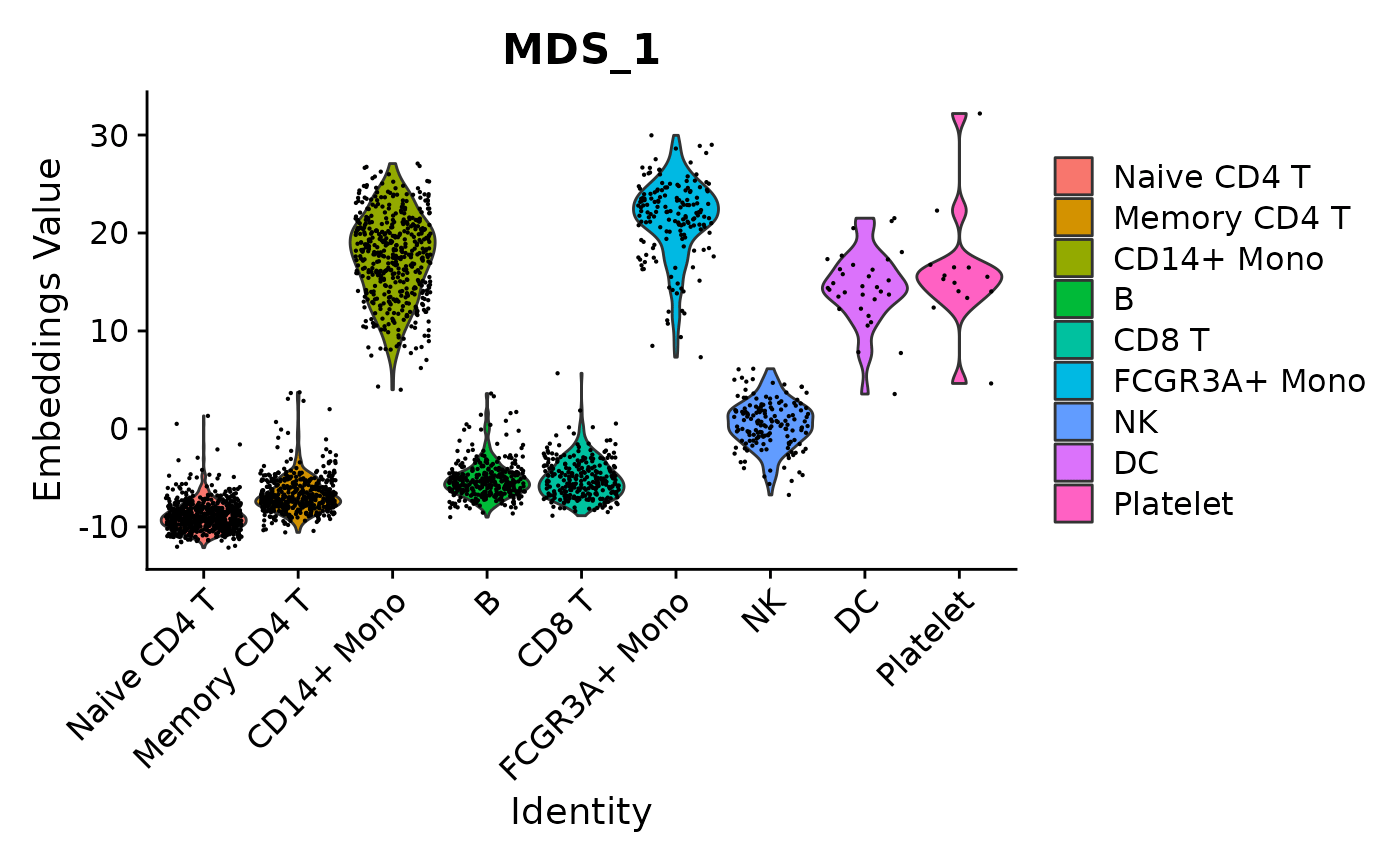
# Explore how the first MDS dimension is distributed across clusters
VlnPlot(pbmc, features = "MDS_1")
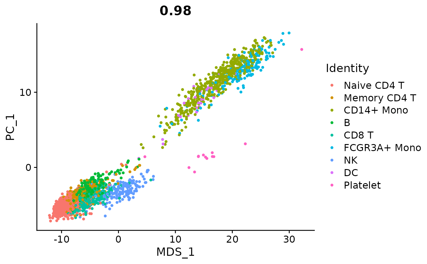
# See how the first MDS dimension is correlated with the first PC dimension
FeatureScatter(pbmc, feature1 = "MDS_1", feature2 = "PC_1")
Session Info
## R version 4.2.0 (2022-04-22)
## Platform: x86_64-pc-linux-gnu (64-bit)
## Running under: Ubuntu 20.04.5 LTS
##
## Matrix products: default
## BLAS:   /usr/lib/x86_64-linux-gnu/openblas-pthread/libblas.so.3
## LAPACK: /usr/lib/x86_64-linux-gnu/openblas-pthread/liblapack.so.3
##
## locale:
##  [1] LC_CTYPE=en_US.UTF-8       LC_NUMERIC=C
##  [3] LC_TIME=en_US.UTF-8        LC_COLLATE=en_US.UTF-8
##  [5] LC_MONETARY=en_US.UTF-8    LC_MESSAGES=en_US.UTF-8
##  [7] LC_PAPER=en_US.UTF-8       LC_NAME=C
##  [9] LC_ADDRESS=C               LC_TELEPHONE=C
## [11] LC_MEASUREMENT=en_US.UTF-8 LC_IDENTIFICATION=C
##
## attached base packages:
## [1] stats     graphics  grDevices utils     datasets  methods   base
##
## other attached packages:
##  [1] ggplot2_3.4.1                 thp1.eccite.SeuratData_3.1.5
##  [3] stxBrain.SeuratData_0.1.1     ssHippo.SeuratData_3.1.4
##  [5] pbmcsca.SeuratData_3.0.0      pbmcMultiome.SeuratData_0.1.2
##  [7] pbmc3k.SeuratData_3.1.4       panc8.SeuratData_3.0.2
##  [9] ifnb.SeuratData_3.1.0         hcabm40k.SeuratData_3.0.0
## [11] bmcite.SeuratData_0.3.0       SeuratData_0.2.2
## [13] SeuratObject_4.1.3            Seurat_4.3.0
##
## loaded via a namespace (and not attached):
##   [1] systemfonts_1.0.4      plyr_1.8.8             igraph_1.4.1
##   [4] lazyeval_0.2.2         sp_1.6-0               splines_4.2.0
##   [7] listenv_0.9.0          scattermore_0.8        digest_0.6.31
##  [10] htmltools_0.5.4        fansi_1.0.4            magrittr_2.0.3
##  [13] memoise_2.0.1          tensor_1.5             cluster_2.1.3
##  [16] ROCR_1.0-11            globals_0.16.2         matrixStats_0.63.0
##  [19] pkgdown_2.0.7          spatstat.sparse_3.0-0  colorspace_2.1-0
##  [22] rappdirs_0.3.3         ggrepel_0.9.3          textshaping_0.3.6
##  [25] xfun_0.37              dplyr_1.1.0            crayon_1.5.2
##  [28] jsonlite_1.8.4         progressr_0.13.0       spatstat.data_3.0-0
##  [31] survival_3.3-1         zoo_1.8-11             glue_1.6.2
##  [34] polyclip_1.10-4        gtable_0.3.1           leiden_0.4.3
##  [37] future.apply_1.10.0    abind_1.4-5            scales_1.2.1
##  [40] spatstat.random_3.1-3  miniUI_0.1.1.1         Rcpp_1.0.10
##  [43] viridisLite_0.4.1      xtable_1.8-4           reticulate_1.28
##  [46] htmlwidgets_1.6.1      httr_1.4.5             RColorBrewer_1.1-3
##  [49] ellipsis_0.3.2         ica_1.0-3              farver_2.1.1
##  [52] pkgconfig_2.0.3        sass_0.4.5             uwot_0.1.14
##  [55] deldir_1.0-6           utf8_1.2.3             tidyselect_1.2.0
##  [58] labeling_0.4.2         rlang_1.0.6            reshape2_1.4.4
##  [61] later_1.3.0            munsell_0.5.0          tools_4.2.0
##  [64] cachem_1.0.7           cli_3.6.0              generics_0.1.3
##  [67] ggridges_0.5.4         evaluate_0.20          stringr_1.5.0
##  [70] fastmap_1.1.1          yaml_2.3.7             ragg_1.2.5
##  [73] goftest_1.2-3          knitr_1.42             fs_1.6.1
##  [76] fitdistrplus_1.1-8     purrr_1.0.1            RANN_2.6.1
##  [79] pbapply_1.7-0          future_1.31.0          nlme_3.1-157
##  [82] mime_0.12              formatR_1.14           compiler_4.2.0
##  [85] plotly_4.10.1          png_0.1-8              spatstat.utils_3.0-1
##  [88] tibble_3.1.8           bslib_0.4.2            stringi_1.7.12
##  [91] highr_0.10             desc_1.4.2             lattice_0.20-45
##  [94] Matrix_1.5-3           vctrs_0.5.2            pillar_1.8.1
##  [97] lifecycle_1.0.3        spatstat.geom_3.0-6    lmtest_0.9-40
## [100] jquerylib_0.1.4        RcppAnnoy_0.0.20       data.table_1.14.8
## [103] cowplot_1.1.1          irlba_2.3.5.1          httpuv_1.6.9
## [106] patchwork_1.1.2        R6_2.5.1               promises_1.2.0.1
## [109] KernSmooth_2.23-20     gridExtra_2.3          parallelly_1.34.0
## [112] codetools_0.2-18       MASS_7.3-56            rprojroot_2.0.3
## [115] withr_2.5.0            sctransform_0.3.5      parallel_4.2.0
## [118] grid_4.2.0             tidyr_1.3.0            rmarkdown_2.20
## [121] Rtsne_0.16             spatstat.explore_3.0-6 shiny_1.7.4